Sentry Page Protection
Data Analysis [1-15]
Proc Univariate
The first step to data analysis is to look at the shape and distribution of the data.
This can be done by using Proc Univariate.
Example
Copy and run the DEMO data set from the yellow box below.
The first step to data analysis is to look at the shape and distribution of the data.
This can be done by using Proc Univariate.
Example
Copy and run the DEMO data set from the yellow box below.
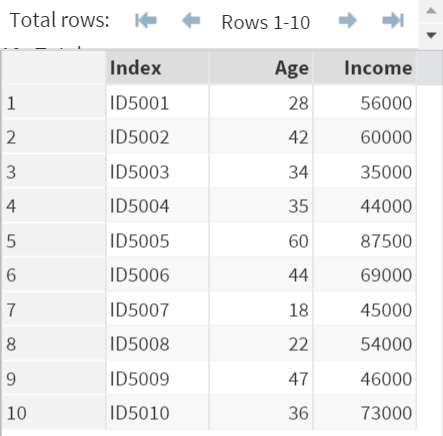
The DEMO data set contains a list of event participants along with their age and income.
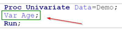
Now, enter and run the code below on SAS Studio:
Example
Proc Univariate Data=Demo;
Var Age;
Run;
By default, Proc Univariate displays 5 sets of statistics:
1. Moment
In statistics, a moment is a measure of the shape of the data.
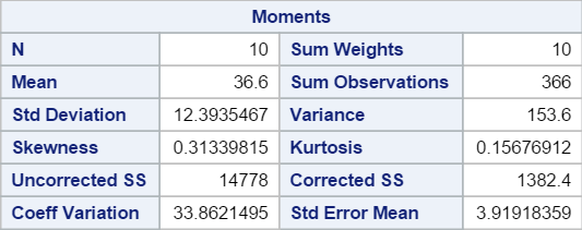
The first four moments are:
- 1st: Mean
- 2nd: Variance
- 3rd: Skewness
- 4th: Kurtosis
In our example, all four moments are listed in the first table.
2. Basic Statistical Measures
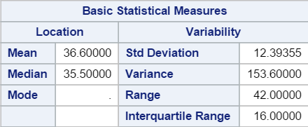
The second table shows the basic statistical measures such as:
- Mean
- Median
- Mode
- Standard Deviation
- Variance
- Range
- Interquartile Range
3. Tests for Location
The tests for location are the hypothesis testings on whether the population mean is significantly different from zero.
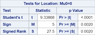
The three tests for locations are:
- Student’s test
- sign test
- Wilcoxon signed rank test
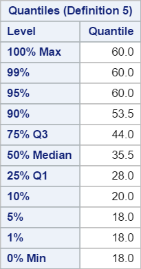
4. Quantiles
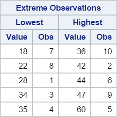
5. Extreme Observations
The statistics give us a good idea of how the data is distributed.
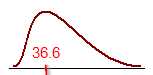
The average age of the events participant is 36.6 with the standard deviation of 12.4.
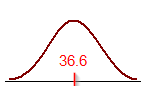
The skewness is 0.3133, which shows the distribution being slightly skewed to the right.
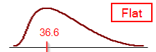
The kurtosis is 0.1568. This indicates a "flat" distribution as opposed to a "peak" one.
Understanding the distribution of the data is an essential step prior to performing the more complex statistical analysis.
Proc Univariate is a quick way to do just that!
Proc Univariate is a quick way to do just that!
Exercise
Take a look at the DEMO data set again.
Run Proc Univariate on the INCOME variable.
Briefly describe the distribution of the INCOME.
Take a look at the DEMO data set again.
Run Proc Univariate on the INCOME variable.
Briefly describe the distribution of the INCOME.
Need some help?
HINT:
Simply use the code covered in this session as a template and you should get the correct results.
SOLUTION:
Proc Univariate Data=Demo;
Var Income;
Run;
The average income of this population is $56,950 with a standard deviation of about $16,000.
The distribution is slightly skewed to the right (skewness: 0.6472)
The negative kurtosis (-0.0276) indicates a flat distribution.
The highest and lowest incomes are $87,500 and $35,000, respectively. The extreme incomes don't seem to be too far off from the mean at $56,950.
Fill out my online form.