Time Series Modeling
[3-10]
[3-10]
Before we fit any time series model on our data, let's properly create the time variable for the x-axis.
If you haven't created the SALES data set, copy and run the code from the yellow box below:
The data about the time are captured in the MONTH, WEEK and DAY columns:
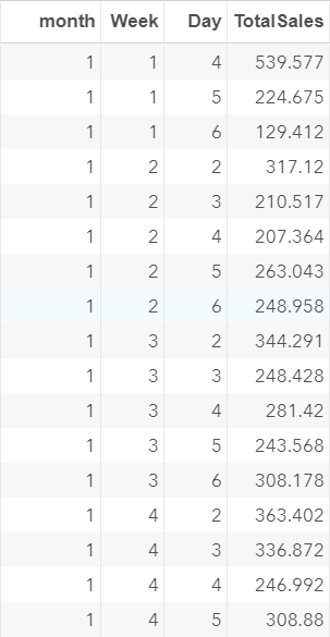
We can clearly identify the time point of each observations.
However, in order to perform any type of time series modeling, we need to create a single time column that captures the sequential order of each time point.
One way to create such a column is to convert the DAY, WEEK and MONTH columns into a SAS date column and use it as our x-axis.
Below is the code that we run to create the TIME column:
data sales2;
set sales;
cumweek = week + 4*(month-1);
time = day + 7*(cumweek-1);
run;
data day_temp;
do time = 4 to 90;
output;
end;
run;
data sales3;
merge day_temp sales2;
by time;
drop cumweek;
run;
set sales;
cumweek = week + 4*(month-1);
time = day + 7*(cumweek-1);
run;
data day_temp;
do time = 4 to 90;
output;
end;
run;
data sales3;
merge day_temp sales2;
by time;
drop cumweek;
run;
The breakdown of the code will be explained shortly.
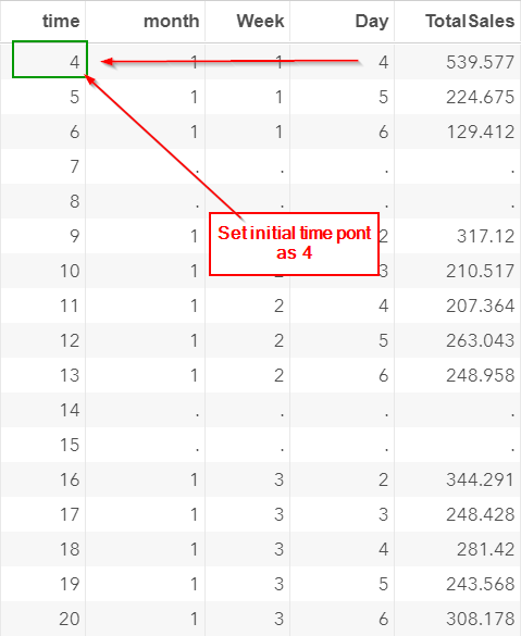
Let's open the SALES3 data set and look at the TIME column that we created:

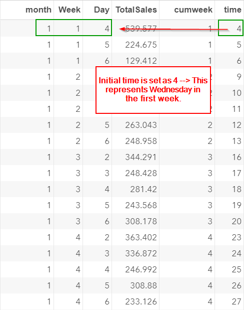
The initial time point in the TIME column is set as 4.
This represents the Day 4 (Wednesday) of the first week of the month.
Let's look at the time on a calendar:
Note: the initial time point does not matter. The time column works as long as it is in sequential order that reflects the weekly pattern from the data.
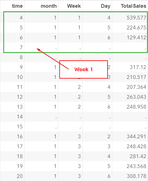
Let's look at the first four observations.
These are the sales record in week 1:
Important:
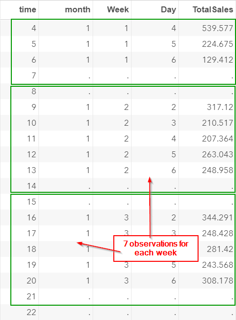
We also include additional rows for the weekends and holidays as well:
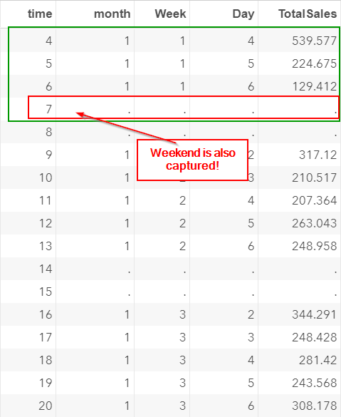
The sales for the weekends (and holidays) are set as missing.
Including the weekends and holidays in the TIME column ensures that weekly pattern is reflected in the x-axis.
Except for the very first week, each week has exactly seven observations:
Now, let's look at the breakdown of the code to create this TIME column.
The code contains three data steps.
In the first data step, we created the TIME column:
data sales2;
set sales;
cumweek = week + 4*(month-1);
time = day + 7*(cumweek-1);
run;
set sales;
cumweek = week + 4*(month-1);
time = day + 7*(cumweek-1);
run;
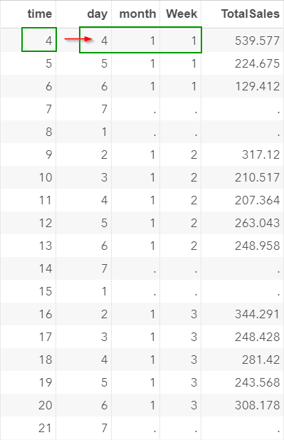
The initial value of the TIME column is set as 4.
This represents Day 4 (Wednesday) in the first week:
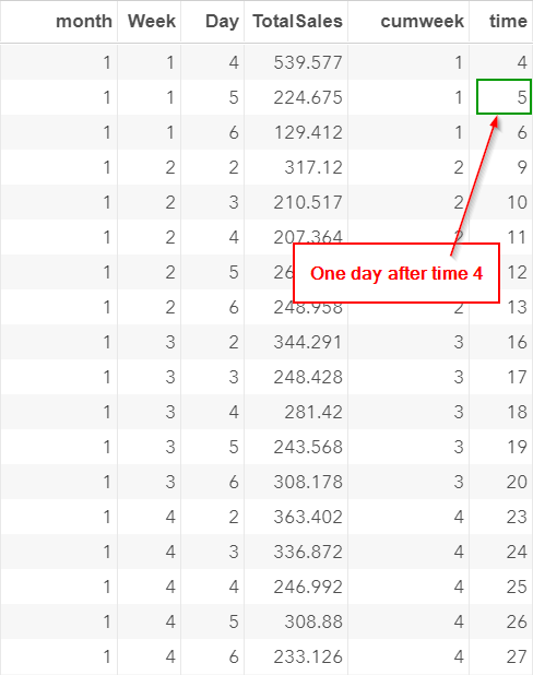
On the next day, the TIME value is set as 5.
This reflects that fact that day 5 in the first week is one day after the day 4 in the same week.

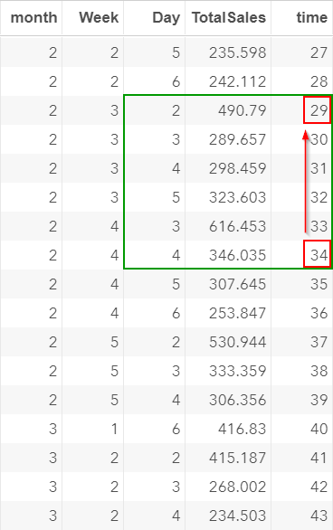
Time 29 is a Monday:
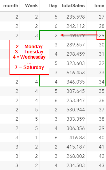
In the previous section, we learned that there is a seasonal spike (i.e. higher sales) on Monday.
When modeling the data, we would expect that there is also a spike at time 34 (which is five periods after day 29):
However, due to the missing values, time 34 is actually a Wednesday!
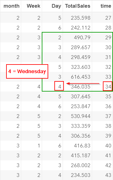
Treating each observation as an individual time point changes the seasonal pattern of the data.
This will affect the model that we are going to build.
A better way to create the time variable is to create a sequential date column that matches the weekday from (1=Sunday to 7=Saturday).
Let's look at an example.
The breakdown of the code can be found here.
The TIME column created begins at time 4.
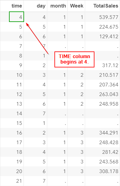
It corresponds to the time point at Day 4 of the very first week.
Data are collected starting on a Wednesday.
Time 4-7 represents the sales record from Wednesday to Saturday in the very first week:
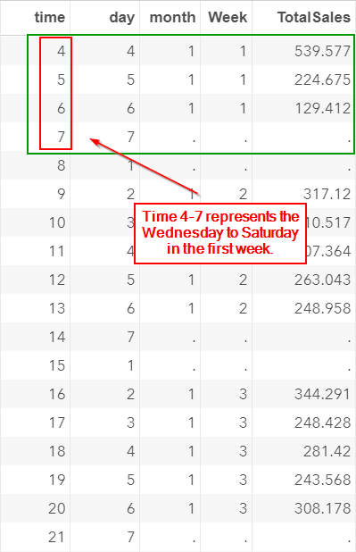
Note: Saturday is a holiday and the totalsales are set as missing.
This row is also included in the data set:
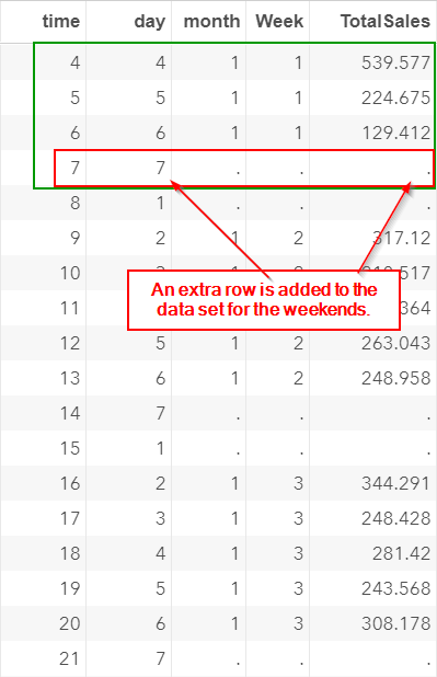
Similarly, time 8-14 represents the second week of the data.
It goes from (1=Sunday) to (7=Saturday):

Similarly, additional rows are added for the weekends:
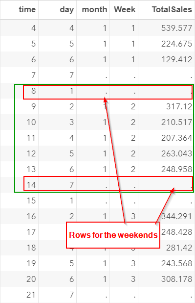
The data set is now structured by weeks of 7 days (except for the very first week).
Let's scroll down to the weeks that contain holiday(s).
Time 43-49 represents the third week of month two:
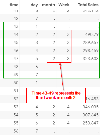
The Friday in this week is a holiday. The store is closed.
However, an additional row is added to the data set as well:
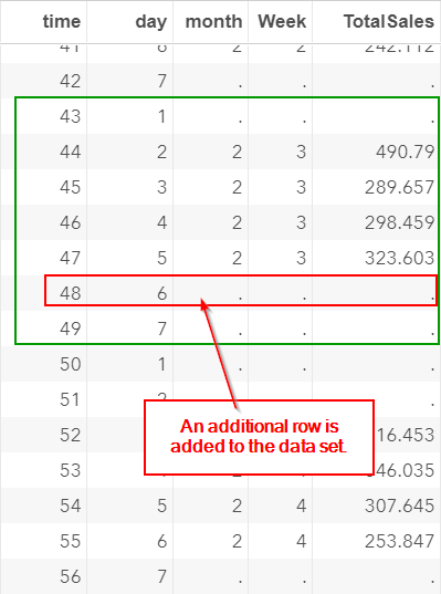
The TIME column is structured in a group of 7 days (except for the very first week).
Whether the week contains weekends or holidays, there are 7 rows of data for the week.
The benefits of creating the TIME column in such a way is that the seasonal pattern can be modeled every seven periods.
The seasonal pattern is now incorporated into the TIME column.
Exercise
Are there any significant difference in sales between the different week of the month?
Create a frequency table for the total sales for each week of the month.
In addition, fit an ANOVA model and test the difference in sales between five weeks of the month.
Are there any significant difference in sales between the different week of the month?
Create a frequency table for the total sales for each week of the month.
In addition, fit an ANOVA model and test the difference in sales between five weeks of the month.
Need some help?
Fill out my online form.