Time Series Modeling
[3-10]
[3-10]
Properly setting up the time variable for the x-axis is crucial to your time series analysis.
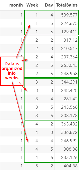
Before we go ahead and create the time variable, let's take a look at how the data is structured.
If you haven't created the SALES data set, copy and run the code from the yellow box below:
Except for the very first week, the sales data is organized into weeks of five days:
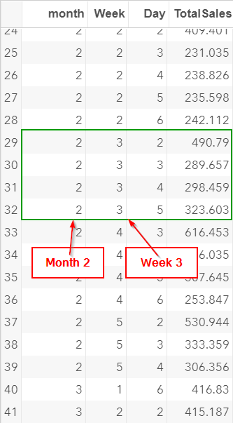
If you scroll down, you will notice that some weeks are missing a day or two.
Let's scroll down to the week 3 in month 2:
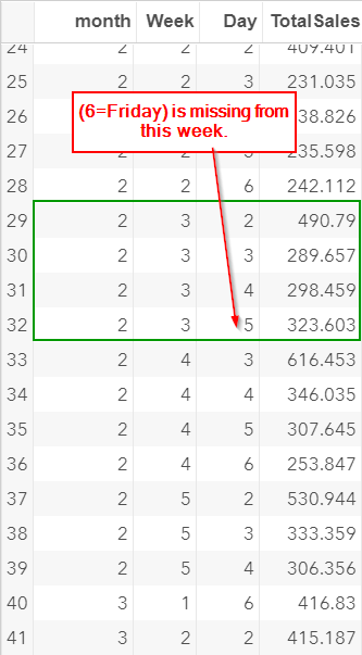
There are only four days in this week. There is no sales record for Friday.
In addition, the following week is missing sales record for Monday as well.
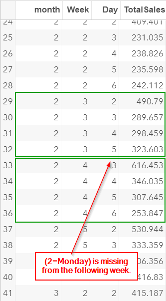
The missing records are likely due to holidays.
The store is closed and there is no sales record for these days.
Creating the Time Variable
Now, there are a number of ways to create the time variable.
The simplest way to create the variable is to treat each observation as an independent time point.
Let's look at an example.
data sales2;
set sales;
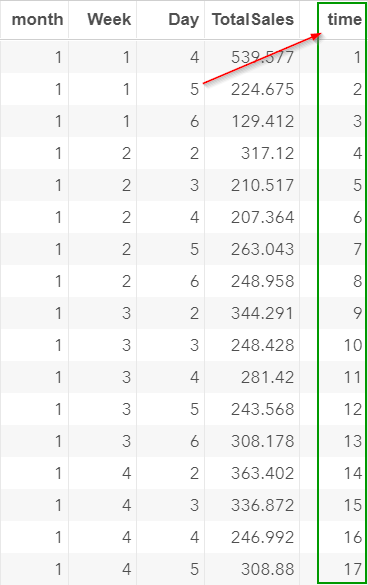
time = _n_;
run;
set sales;
time = _n_;
run;
This creates a TIME variable that goes up from one to 60:
The problem with treating each observation as an individual time point is that the time variable created does not reflect the seasonal pattern of the data.
Let's look at time 29 to 34:
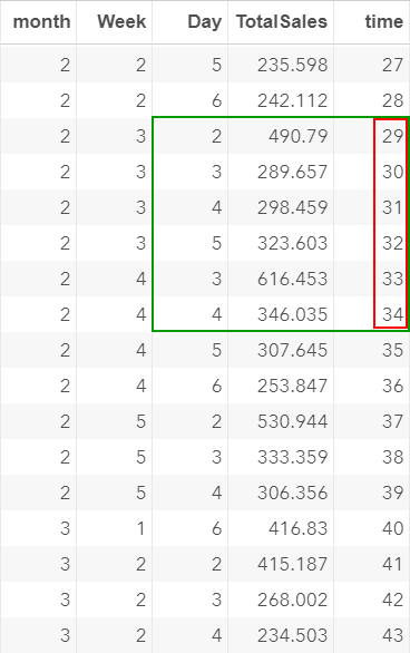
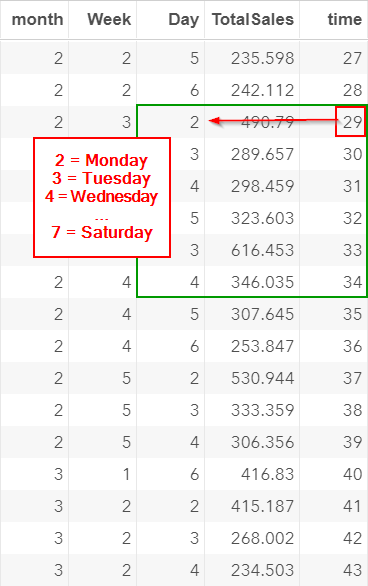
Time 29 is a Monday:
In the previous section, we learned that there is a seasonal spike (i.e. higher sales) on Monday.
When modeling the data, we would expect that there is also a spike at time 34 (which is five periods after day 29):

However, due to the missing values, time 34 is actually a Wednesday!
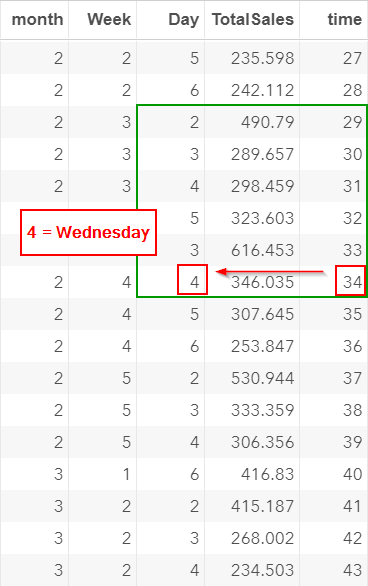
Treating each observation as an individual time point changes the seasonal pattern of the data.
This will affect the model that we are going to build.
A better way to create the time variable is to create a sequential date column that matches the weekday from (1=Sunday to 7=Saturday).
Let's look at an example.
data sales2;
set sales;
weekno = week + 4*(month-1);
time = day + 7*(weekno-1);
drop weekno;
run;
data time_temp;
do time = 4 to 90;
day = mod(time, 7);
if day = 0 then day = 7;
output;
end;
run;
data sales3;
merge time_temp sales2;
by time;
drop month week;
run;
set sales;
weekno = week + 4*(month-1);
time = day + 7*(weekno-1);
drop weekno;
run;
data time_temp;
do time = 4 to 90;
day = mod(time, 7);
if day = 0 then day = 7;
output;
end;
run;
data sales3;
merge time_temp sales2;
by time;
drop month week;
run;
The breakdown of the code can be found here.
The TIME column created begins at time 4.

It corresponds to the time point at Day 4 of the very first week.
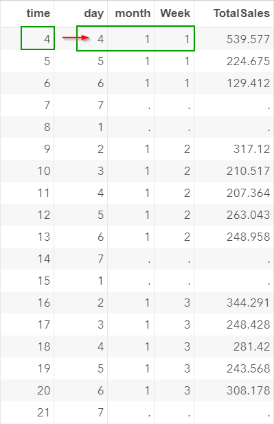
Data are collected starting on a Wednesday.
Time 4-7 represents the sales record from Wednesday to Saturday in the very first week:
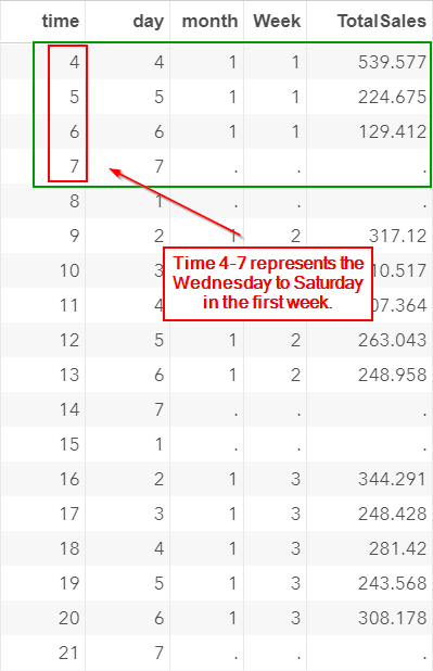
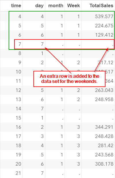
Note: Saturday is a holiday and the totalsales are set as missing.
This row is also included in the data set:
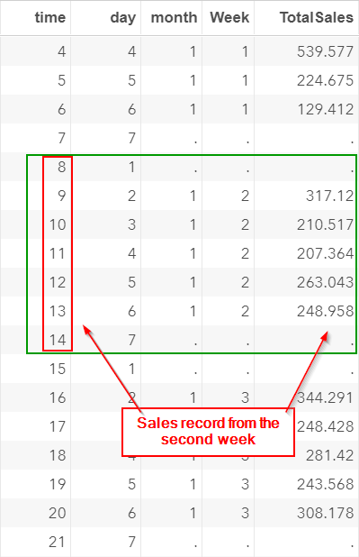
Similarly, time 8-14 represents the second week of the data.
It goes from (1=Sunday) to (7=Saturday):
Similarly, additional rows are added for the weekends:
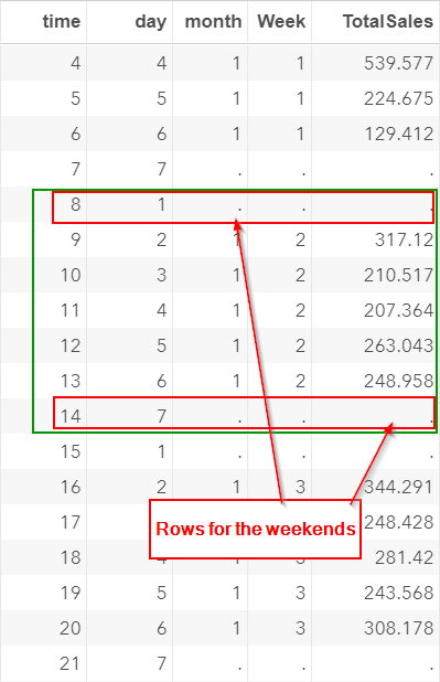
The data set is now structured by weeks of 7 days (except for the very first week).
Let's scroll down to the weeks that contain holiday(s).
Time 43-49 represents the third week of month two:
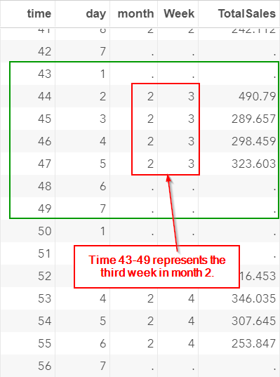
The Friday in this week is a holiday. The store is closed.
However, an additional row is added to the data set as well:

The TIME column is structured in a group of 7 days (except for the very first week).
Whether the week contains weekends or holidays, there are 7 rows of data for the week.
The benefits of creating the TIME column in such a way is that the seasonal pattern can be modeled every seven periods.
The seasonal pattern is now incorporated into the TIME column.
Exercise
Are there any significant difference in sales between the different week of the month?
Create a frequency table for the total sales for each week of the month.
In addition, fit an ANOVA model and test the difference in sales between five weeks of the month.
Are there any significant difference in sales between the different week of the month?
Create a frequency table for the total sales for each week of the month.
In addition, fit an ANOVA model and test the difference in sales between five weeks of the month.
Need some help?
Fill out my online form.