Time Series Modeling
[4-10]
[4-10]
Time series forecasting is about using the past data to predict the future.
However, does the past value really have any forecasting power on the future?
If the sales on Tuesday is $300, should we expect the sales on Wednesday to be roughly the same?
What about the sales on Thursday?
In order to build a good model for sales forecasting, we must learn more about the relationship between the sales at the different time point.
Let's look at an example.
The DS data set contains the price of a stock over a period of 300 days.
Now, we'd like to look at the relationship between the stock price at two consecutive time point.
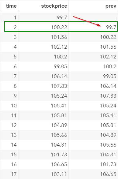
We will create another column called PREV which contains the stock price on the previous day.
The LAG function is used:
data ds2;
set ds;
prev = lag(stockprice);
run;
set ds;
prev = lag(stockprice);
run;
For example, the stock price at time 2 is $100.22. The previous day's price (i.e. time 1) is $99.7.
We want to look at how the prices on two consecutive days are correlated with each other.
We will treat these two columns as two separate columns and compute the autocorrelation between them.
SAS does not have a built-in option to calculate the autocorrelation.
Below is the macro that does the calculation:
%macro autocorr (in=,var=,lag=);
proc sql noprint;
select mean(&var) into :average from ∈
quit;
data autocorr;
set &in end=eof;
a = &var;
c = lag&lag.(a);
a1 = (a-&average);
a2 = (c-&average);
a3 = a1*a2;
a4 = (a-&average)**2;
s3 + a3;
s4 + a4;
r = s3/s4;
if eof = 1;
keep r;
run;
%mend;
proc sql noprint;
select mean(&var) into :average from ∈
quit;
data autocorr;
set &in end=eof;
a = &var;
c = lag&lag.(a);
a1 = (a-&average);
a2 = (c-&average);
a3 = a1*a2;
a4 = (a-&average)**2;
s3 + a3;
s4 + a4;
r = s3/s4;
if eof = 1;
keep r;
run;
%mend;
Note: the macro itself does not generate any result. It is simply a memory of the code that can be executed once it is called.
Now, let's call the AUTOCORR macro that we have just created.
%autocorr(in=ds, var=stockprice, lag=1);
Calling the macro is easy!
You just have to specify the three things below:
- IN: the input data set. In our example, it is the DS data set.
- VAR: the variable of interest. In our example, it is the variable STOCKPRICE.
- LAG: the number of lag you want to compute for the autocorrelation.
Note: the macro is quite versatile. It can calculate the autocorrelation for more than one lag. We will look at some examples shortly.
The macro computes the autocorrelation between the current day's stock price and the previous day's stock price.
The autocorrelation is 0.9807.
That's a very high correlation between the stock prices on two consecutive days!
This is important.
When performing the forecasting, this is a hint that the stock price on the previous day is highly correlated with the current stock price that you want to forecast.
Now, what about the correlation between the stock price and the price from two days prior?
Maybe the price from two days ago are also correlated with the current day's price?
This is worth investigating.
We will use the AUTOCORR macro to compute the autocorrelation between the current stock price and the price from two days prior.
Simply set LAG=2 in the third parameter of the AUTOCORR macro:
%autocorr(in=ds, var=stockprice, lag=2);
The autocorrelation between the current stock price and the price from two days prior is 0.9612.
This is still a very strong correlation, although it is less strong than the autocorrelation at lag 1.
The correlation isn't as strong as with the one-lagged value (i.e. r=0.5636).
Maybe we should put more weight on the closer time period than the future time period when performing the forecasting.
This is the idea how you build the forecasting model.
We have just computed the autocorrelation at lag 1 (r=0.5636) and lag 2 (r=0.2389).
However, are these values statistically significant?
Maybe these positive autocorrelation estimations are generated by chance?
Fortunately, we can perform statistical testings to find out whether these values are significant.
ACF Plot
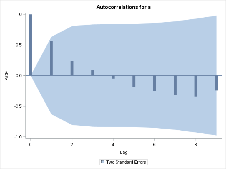
The ACF plot shows the autocorrelation of each lag on the plot.
You can create such a plot using the TIMESERIES procedure.
proc timeseries data=ds plots=acf;
var a;
run;
var a;
run;
The procedure above creates the ACF plot below:
If you look at the bar at lag 1 and lag 2, the results match our calculations earlier.
The autocorrelation is 0.5636 at lag 1 and 0.2389 at lag 2:
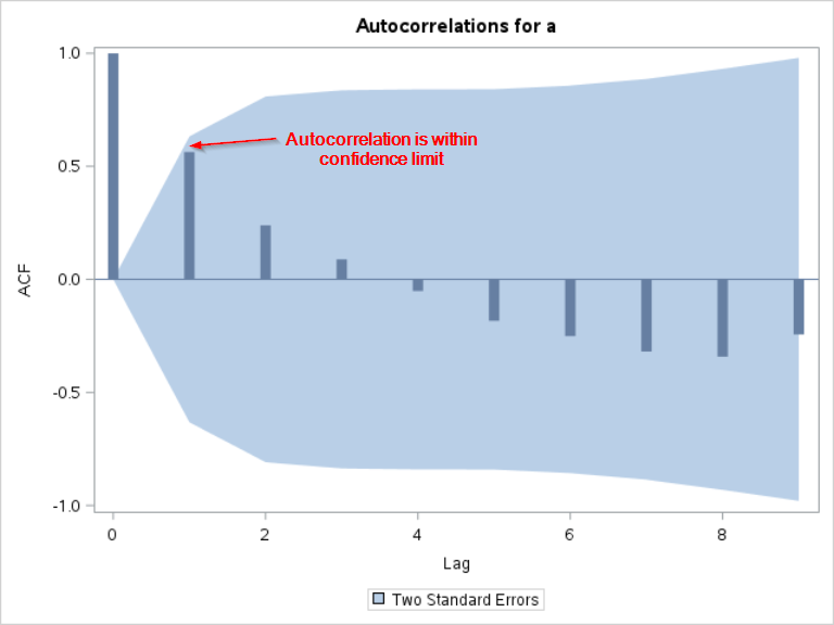
The ACF plot also shows the confidence interval.
Although the autocorrelation at lag 1 is fairly high (r=0.5636), we cannot conclude that the autocorrelation is significant since it is still within the confidence interval.
There is no significant autocorrelation on the ACF plot.
The current value does not seem to be significantly correlated with any of its lagged values.
Let's go back to the SALES3 data set and plot the ACF plot for the TOTALSALES column.
proc timeseries data=sales3 plots=acf;
id time interval=day format=best.;
var totalsales;
run;
id time interval=day format=best.;
var totalsales;
run;
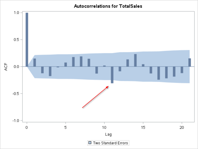
The ACF shows a spike at lag 11:
We can also look at the standardized ACF plot:
The plot shows a spike that is significant at lag 11.
This indicates that the sales today is significantly correlated with the sales from 11 days ago.
This is quite unexpected.
This information will be useful when we build our final model.
In the next section, we will look at a few more examples of the ACF plots.
Exercise
Are there any significant difference in sales between the different week of the month?
Create a frequency table for the total sales for each week of the month.
In addition, fit an ANOVA model and test the difference in sales between five weeks of the month.
Are there any significant difference in sales between the different week of the month?
Create a frequency table for the total sales for each week of the month.
In addition, fit an ANOVA model and test the difference in sales between five weeks of the month.
Need some help?
Fill out my online form.


