Time Series Modeling
[3-10]
[3-10]
Before we fit any time series model to our data, let's properly create the time variable for the x-axis.
If you haven't created the SALES data set, copy and run the code from the yellow box below:
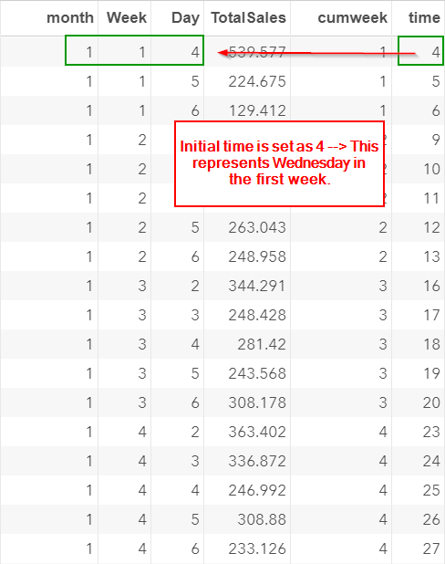
The time point at each observation is captured in the MONTH, WEEK and DAY columns:
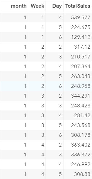
For example, let's look at the very first observation:
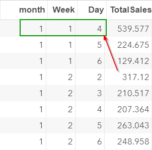
We have:
- Month = 1
- Week = 1
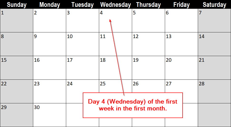
- Day = 4 (Wednesday)
This represents the Wednesday of the first week in the first month.
We can identify the time point of each observations based on these three columns.
However, in order to perform any type of time series modeling, we need to create a single time column that captures the sequential order of each time point.
One way to create such a column is to convert the DAY, WEEK and MONTH columns into a SAS date column and use it as our x-axis.
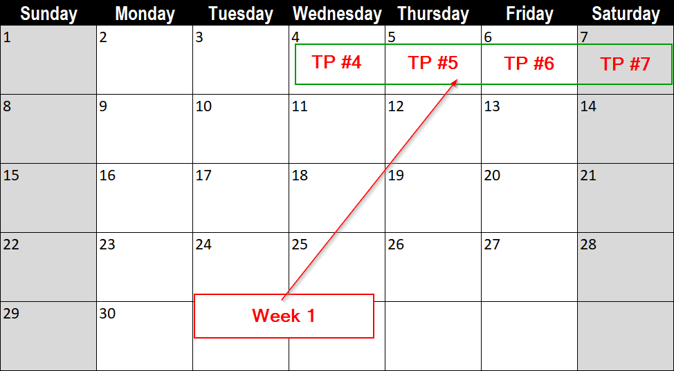
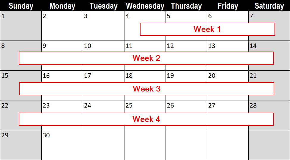
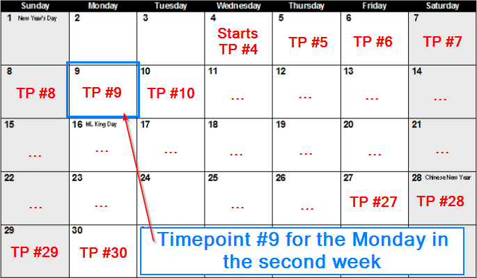
Let's look at the very first time point on a calendar.
The sales began to be recorded on the Wednesday of the first week of the month:
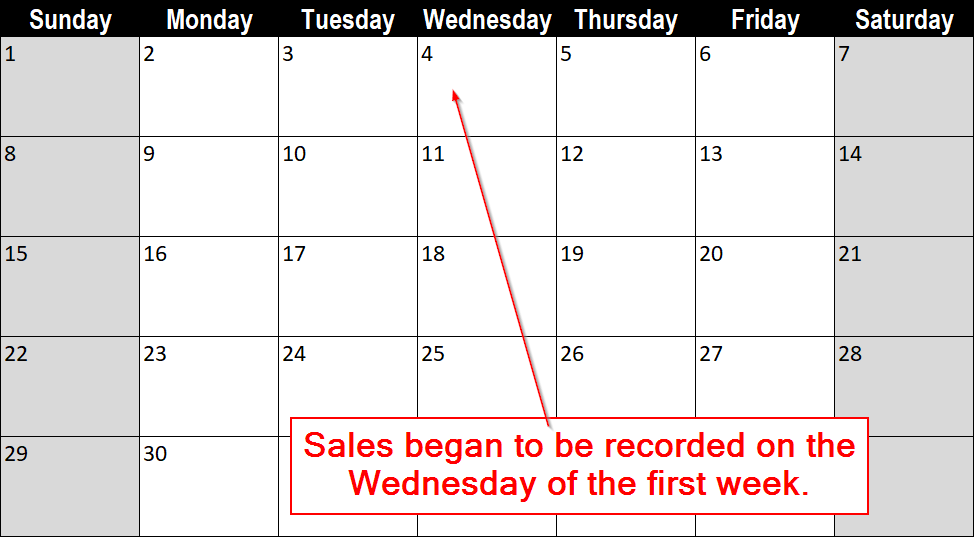
This is going to be our initial time point:
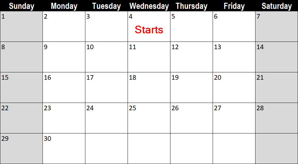
Logically, we are going to set this as our timepoint #1.
However, we will set this as timepoint #4 instead.
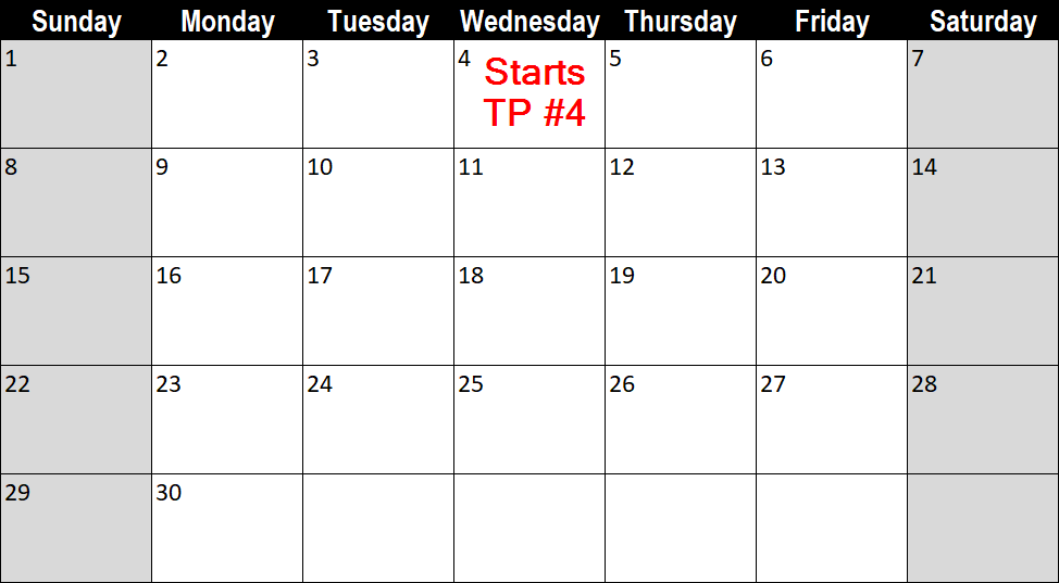
It really does not matter whether you set this as timepoint #1 or timepoint #4.
We are going to treat this time point as the very first timepoint in this data set.
The timepoint for the next day will be #5.
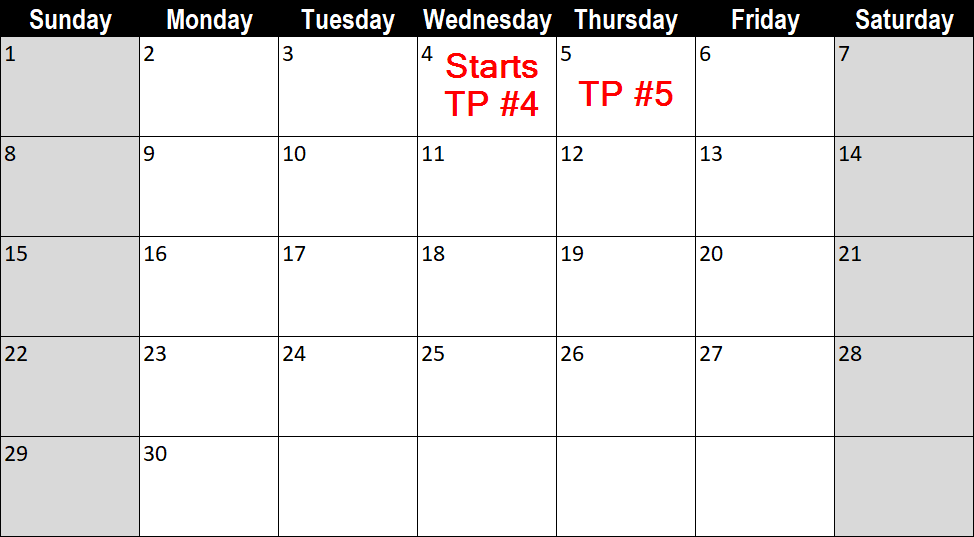
The day after will be timepoint #6, and so forth.
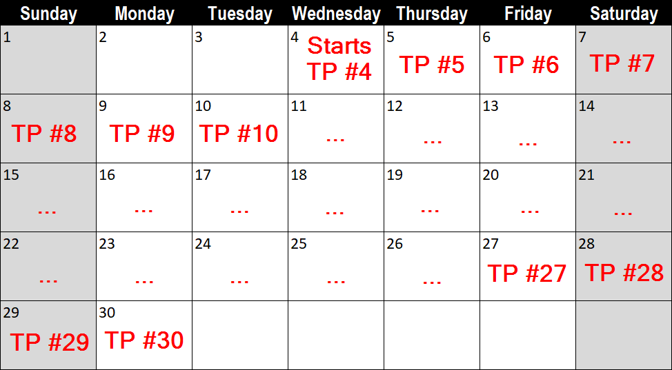
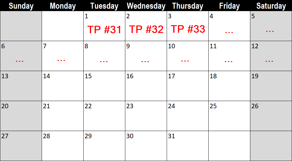
In month 2, the time point will continue at TP #31:
This will continue until all of the observations in our data set are matched with a unique timepoint on the calendar.
Now, the code to generate the these time points are a little tricky.
Run the code from the box below:
data sales2;
set sales;
cumweek = week + 4*(month-1);
time = day + 7*(cumweek-1);
run;
data day_temp;
do time = 4 to 90;
output;
end;
run;
data sales3;
merge day_temp sales2;
by time;
drop cumweek;
run;
set sales;
cumweek = week + 4*(month-1);
time = day + 7*(cumweek-1);
run;
data day_temp;
do time = 4 to 90;
output;
end;
run;
data sales3;
merge day_temp sales2;
by time;
drop cumweek;
run;
The breakdown of the code will be explained shortly.
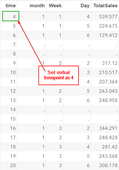
Let's open the SALES3 data set and look at the TIME column that we created:

This is the TIME column that matched what we had on the calendar.
The very first time point is set as 4:
There are four calendar days (i.e. Wednesday, Thursday, Friday, Saturday) in the first week.
These are represented by time point 4 to 7:

Additional rows are also included for the weekends and the holidays. The total sales are set as missing.

Except for the very first week, each week has exactly seven observations:
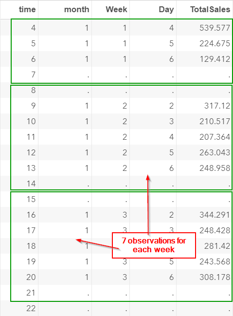
This matched what we had on our calendar:
This will be the TIME column that we are going to use on our x-axis.
Now, let's look at the breakdown of the code to create this TIME column.
The code contains three data steps.
In the first data step, we created the TIME column:
data sales2;
set sales;
cumweek = week + 4*(month-1);
time = day + 7*(cumweek-1);
run;
set sales;
cumweek = week + 4*(month-1);
time = day + 7*(cumweek-1);
run;
The initial value of the TIME column is set as 4.
This represents Day 4 (Wednesday) in the first week:
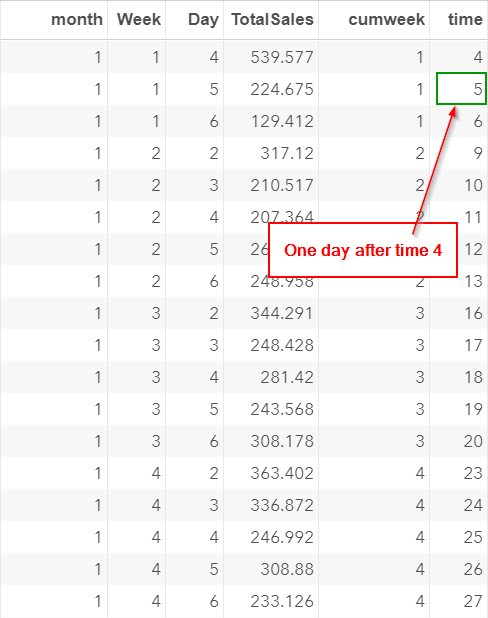
On the next day, the TIME value is set as 5.
The Monday after is set as time point #9.
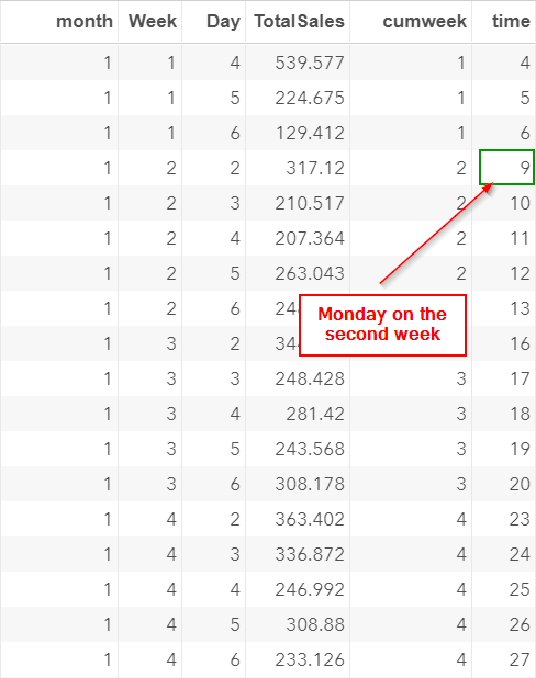
This reflects what we had on our calendar:
The TIME column matches what we had on our calendar.
However, it is missing the weekends and the holidays:
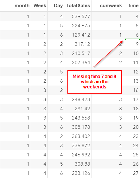
The second and third data steps are to fill in the gaps for the weekends and holidays:
data sales2;
set sales;
cumweek = week + 4*(month-1);
time = day + 7*(cumweek-1);
run;
data day_temp;
do time = 4 to 90;
output;
end;
run;
data sales3;
merge day_temp sales2;
by time;
drop cumweek;
run;
set sales;
cumweek = week + 4*(month-1);
time = day + 7*(cumweek-1);
run;
data day_temp;
do time = 4 to 90;
output;
end;
run;
data sales3;
merge day_temp sales2;
by time;
drop cumweek;
run;
The SALES3 data set will have the time point (i.e. TIME column) listed in numerical order matching the dates on our calendar:

In the next section, we will look at the Autoregression plot which is extremely important for time series analysis.
Exercise
A coworker of yours argues that there is a simpler way to create the time column.
She uses each observation as an individual time point.
Below is her code:
data coworker;
set sales;
time = _n_;
run;
The TIME column is shown below:
A coworker of yours argues that there is a simpler way to create the time column.
She uses each observation as an individual time point.
Below is her code:
data coworker;
set sales;
time = _n_;
run;
The TIME column is shown below:
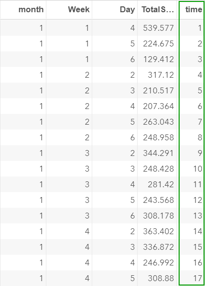
Each individual observation is treated as a unique time point.
The time column goes from 1 to 60 for each of the 60 observations.
Is there any issue using this TIME column on our x-axis?
Why and why not?
Need some help?
Fill out my online form.