Sentry Page Protection
Simple Linear Regression [3-17]
Line of Best Fit
In the last section, we have learned how to explore the relationship between variables on a scatter plot.
We are now going to take a step further and plot a regression line on the scatter plot.
Let's look at the SCHOOL data set again.
Copy and run the code from the yellow line below if you have not done so:
We are now going to take a step further and plot a regression line on the scatter plot.
Let's look at the SCHOOL data set again.
Copy and run the code from the yellow line below if you have not done so:
You can plot the regression line on the scatter plot by using the REG statement within the SGPLOT procedure:
proc sgplot data=school;
reg y=grade10 x=grade9;
run;
reg y=grade10 x=grade9;
run;
You can see the regression line on the plot:
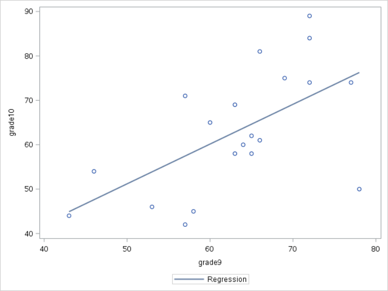
The regression line is called the line of best fit.
It is the line that best fits the data.
How do you define it as the line of "best" fit?
We'll look into that shortly.
Let's first look at the equation of the regression line:
Grade10 = 6.43396 + 0.8952 * Grade9
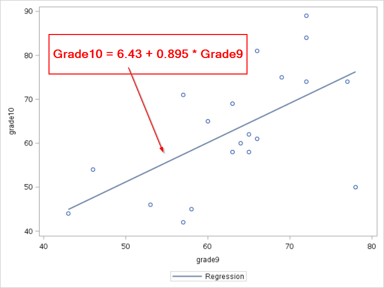
We will show you how to come up with this equation shortly.
The regression line is used to predict the grade 10 result using the grade 9 performance.
Let's look at how well the equation does in the prediction.
We will look at Corrinne as an example:
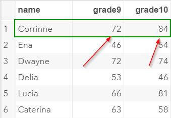
Corrinne had achieved 72 in grade 9 and 84 in grade 10.
She has done pretty well!
If we plug in the grade 9 result in the regression equation, we will have:
Grade10 = 6.43396 + 0.8952 * (72)
Grade10 = 70.88836
Based on the equation, Corrinne is predicted to achieve 70.89 in grade 10. This is quite far off from the observed grade 10 result at 84!
Now, let's look at the difference between the predicted result (70.89) and the observed result (84).
The difference between the two values is 84 - 70.89 = 13.11.
This is called the residual on this particular observation.
Residual measures how far off the predicted value is from the observed value.
Residual is a very important concept for regression analysis.
It allows you to analyze how well the regression does in "fitting" the data.
Now, we are going to compute the residual for each of the 20 observations in the data set.
We will let SAS to do it for us.
proc reg data=school;
id grade9;
model grade10 = grade9 / r;
run;
quit
id grade9;
model grade10 = grade9 / r;
run;
quit
The REG procedure fits a regression line on the SCHOOL data set.
It generates many statistical tables in the output.
For now, we wil scroll down and look at the Output Statistics table:
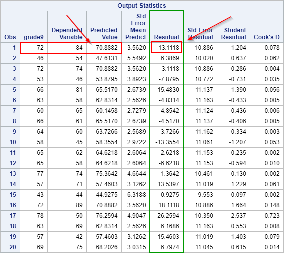
The fifth column of the table contains the list of residuals for each observation.
Simple linear regression works in a similar way but takes a step further.
It formulates an equation that best represents the relationship between the grade 9 and grade 10 results.
E.g.
Grade10 = a + b * Grade9
You then perform a hypothesis testing to find out whether the grade 9 result is a good indicator of the grade 10 performance.
By evaluating and validating the equation parameters (i.e. model), you will be able to make a better prediction on how the student perform in grade 10.
In the next few sections, we will go through the necessary steps to build your first regression model.
Exercise
John is also a new student in grade 10. He achieved 60 in his English class when he was in grade 9.
What would be your best estimate of his result in the English class in grade 10?
You can sort the SCHOOL data set using the code below:
proc sql;
select * from school
order by grade9;
quit;
John is also a new student in grade 10. He achieved 60 in his English class when he was in grade 9.
What would be your best estimate of his result in the English class in grade 10?
You can sort the SCHOOL data set using the code below:
proc sql;
select * from school
order by grade9;
quit;
Need some help?
Fill out my online form.