Sentry Page Protection
Statistical Analysis [3-7]
Paired t-test
A paired t-test can be used to compare the means of two populations where the observations come in pairs.
It is often used when comparing the "before" and "after" results.
Example
It is often used when comparing the "before" and "after" results.
Example
A weight loss product claims to have a significant effect on helping people lose weight.
An independent committee has conducted an inspection and selected 50 healthy participants who have used this particular weight loss product.
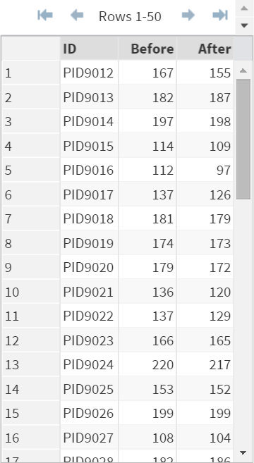
Their weights were measured before and after they have used the product and the results are captured in the INSPECTION data set above.
The INSPECTION data set contains the following variables:
The following hypothesis is being tested:
H0: µd=0
H1: µd≠0
where d = before - after.
Example
Proc ttest Data=Inspection;
Paired Before*After;
Run;
An independent committee has conducted an inspection and selected 50 healthy participants who have used this particular weight loss product.
Their weights were measured before and after they have used the product and the results are captured in the INSPECTION data set above.
The INSPECTION data set contains the following variables:
- ID: Participants' ID
- Before: Weight before using the product
- After: Weight after using the product
The following hypothesis is being tested:
H0: µd=0
H1: µd≠0
where d = before - after.
Example
Proc ttest Data=Inspection;
Paired Before*After;
Run;
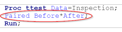
The paired t-test can be done by using Proc ttest with the PAIRED statement.
The PAIRED statement should list the two paired variables separated by an asterisk (*).
Run the program above and the following results will be generated:
1. Basic Statistical Measurements
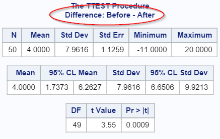
Some basic statistics are generated for the difference between the before- and after- results.
The average weight loss is 4 lbs after using the weight loss product.
The 95% confidence interval is [1.74, 6.26].
We are 95% certain the actual weight loss is between 1.74 to 6.26 lbs.
This rejects the null hypothesis that the difference in weight loss is zero (no effect).
The p-value of 0.0009 also rejects the null hypothesis.
Looks like the weight loss product is indeed effective.
2. Graphs
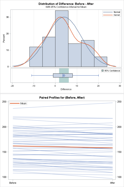
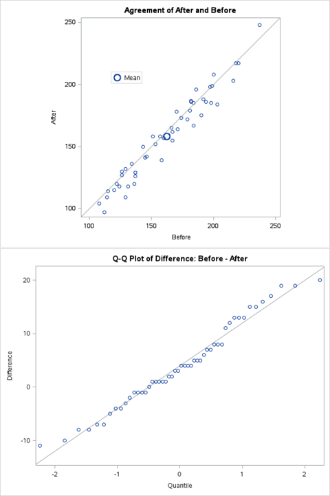
Some of the related graphs such as the histogram and the Q-Q plot are also plotted.
One of the main assumptions for paired t-test is that the difference should be approximately normally distributed.
The linear pattern from the q-q plot suggests the difference is normally distributed.
Exercise
Copy and run the GROUPON data set from the yellow box below:
Copy and run the GROUPON data set from the yellow box below:
The GROUPON data set contains a list of restaurants who have launched a groupon marketing campaign.
A study is conducted to find out if the groupon campaign is profitable for the restaurants.
The data set contains 5 variables:
1. Restaurant
The restaurant identification number
2. N_Bfr
The average number of customers the 3 months prior to the groupon campaign
3. Profit_Bft
The average profit made per customer the 3 months prior to the groupon campaign
4. N_Aftr
The average number of customers the 3 months after to the groupon campaign
5. Profit_Aftr
the average profit made per customer the 3 months after to the groupon campaign
The total profit before and after the groupon campaign can be calculated as:
Total Profit = N x Profit
Where
- N = Average number of customer
- Profit = Average profit per customer
Perform a paired t-test to compare the total profit before and after the groupon campaign.
Is the campaign profitable for the restaurants?
Need some help?
HINT:
First, compute the total profit before and after the campaign. Perform the paired t-test on the total profit after.
SOLUTION:
Data Groupon2;
Set Groupon;
Total_Bfr = N_Bfr*Profit_Bfr;
Total_Aftr = N_Aftr*Profit_Aftr;
Run;
Proc ttest data=groupon2;
paired total_bfr*total_aftr;
Run;
The restaurants, on average, make about $1,900 less after the campaign. The p-value is 0.0001, which demonstrate sufficient evidence that the campaign lowers the total profit for the restaurants.
Fill out my online form.