Sentry Page Protection
Time Series Modeling
[10-15]
[10-15]
Once you have an approximate stationary time series, the next step is to look at the residuals and see if there is any remaining autocorrelation.
If the residual is pure white noise, you're done! All of the correlation is explained by the model (i.e. differencing and transformation).
If not, you might need to add an AR or MA term to correct the autocorrelation before getting to the final model.
Let's look at the following example.
Copy and run the code from the yellow box below:
The TS1 data set contains our usual list of simulated values.
proc arima data=ts1;
identify var=x;
run;
quit;
identify var=x;
run;
quit;
The time series plot shows a non-constant mean:
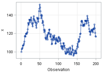
One order of differencing is needed.
proc arima data=ts1;
identify var=x(1);
run;
quit;
identify var=x(1);
run;
quit;
The time series plot looks great after differencing:
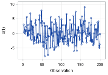
The mean seems to be stabilized with no obvious fluctuation in the variance.
We are now going to look at the ACF and PACF plots:
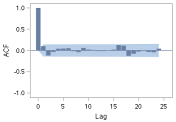
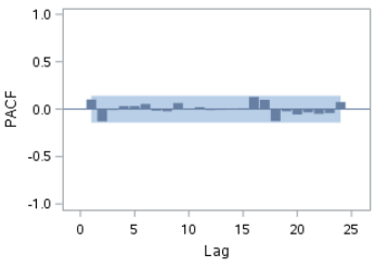
The ACF and PACF plots show no spike at any lag.
The remaining residual (after differencing) looks like white noise.
Now, let's look at the Ljung-box test:
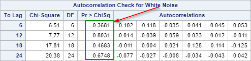
The p-values are above 0.05 at lags 6, 12, 18 and 24.
We conclude that the residuals are white noise.
We're done! All of the correlation seems to have been explained by the differencing.
We have tentatively identified the model to be the ARIMA (0 1 0) model.
Note:
A non-seasonal ARIMA model is usually written in the form of ARIMA (p, d, q) where:
- p = number of AR terms
- d = differencing order
- q = number of MA terms
In our example, the ARIMA (0 1 0) is the model that has one differencing order and no AR and MA term.
Random Walk Model
An ARIMA (0 1 0) model is also called the random-walk model because of its forecasting equation:
Yt - Yt-1 = Wt
where Wt is defined as white noise with a zero mean and constant standard deviation.
If you move Yt-1 to the other side, you will have:
Yt = Yt-1 + Wt
Yt is just a random walk (white noise) away from Yt-1!
In the next few sections, we will look at a number of examples where an AR or MA term is needed to correct the remaining autocorrelation in the residual.
Exercise
Copy and run the STOCKS data set from the yellow box below:
Copy and run the STOCKS data set from the yellow box below:
The STOCKS data set contains a list of stock closing prices for 100 days.
Perform one order of differencing to stabilize the mean and check the Ljung-box test results.
Can you conclude that the residuals are purely white noise?
Need some help?
Fill out my online form.