Sentry Page Protection
Time Series Modeling
[13-15]
[13-15]
We have now learned how to identify the ARIMA model for the time series.
Let's do some forecasting based on the models that we built.
Copy and run the code from the yellow box below:
In section 11, we have identified the model for the TS2 data set to be the ARIMA (1 1 0) model.
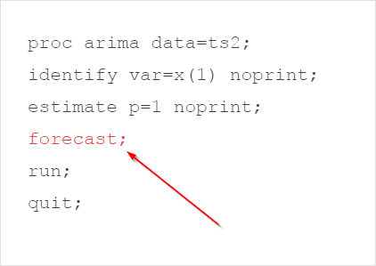
Forecasting can be done by simply adding a FORECAST statement in the ARIMA model.
proc arima data=ts2;
identify var=x(1) noprint;
estimate p=1 noprint;
forecast;
run;
quit;
identify var=x(1) noprint;
estimate p=1 noprint;
forecast;
run;
quit;
The FORECAST statement tells SAS to perform the time series forecasting.
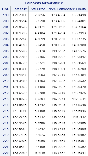
The forecasting table for the next 24 periods (default) is displayed:
How accurate is the forecasting? This is a question a time series forecaster needs to know.
One way to examine the forecasting model is to compare the predicted values and the actual values.
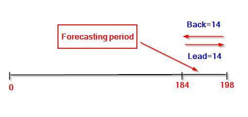
We are going to perform the multi-step forecasting on the last 14 observations.
proc arima data=ts2 plots=(forecast(all));
identify var=x(1) noprint;
estimate p=1 noprint;
forecast back=14 lead=14;
run;
quit;
identify var=x(1) noprint;
estimate p=1 noprint;
forecast back=14 lead=14;
run;
quit;
The BACK=14 option moves back 14 time points for the multi-step forecasting.
The LEAD=14 option tells SAS to perform the multistep forecasting for the last 14 observations.
The PLOTS option tells SAS to plot all of the forecasting values:
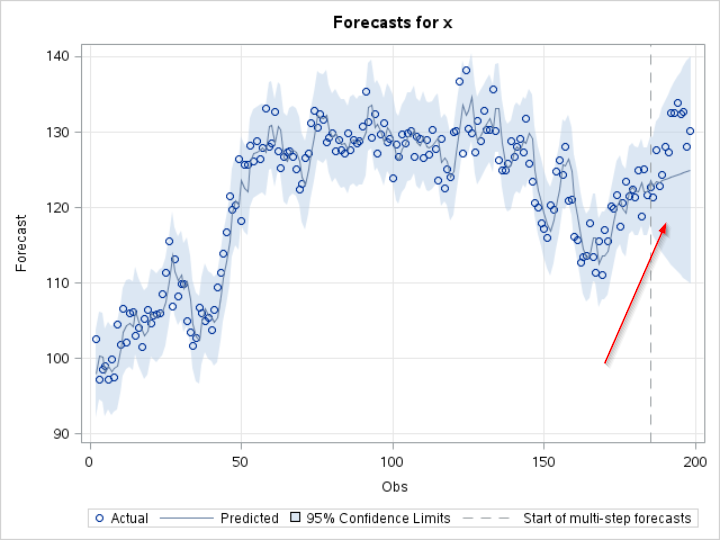
You can visualize the comparison between the predicted values and the actual values.
MAE and RMSE
The MAE and RMSE are two commonly used statistics to check the prediction accuracy.
Proc ARIMA does not have any built-in options to compute the MAE and RMSE.
We will first create an output data set that contains the predicted values and the actual values.
proc arima data=ts2 plots=(forecast(all)) out=forecast;
identify var=x(1) noprint;
estimate p=1 noprint;
forecast back=14 lead=14;
run;
quit;
identify var=x(1) noprint;
estimate p=1 noprint;
forecast back=14 lead=14;
run;
quit;
The OUT=FORECAST option creates an output data set called FORECAST:
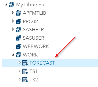
The FORECAST data set contains the column X as well as the predicted values of X.
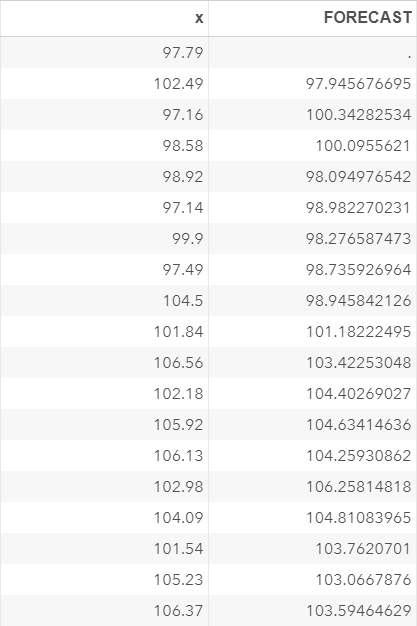
Now, we are going to compute the MAE and RMSE using the last 14 observations of the FORECAST data set.
data test;
set forecast;
if _n_ > 184;
run;
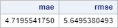
proc sql;
select mean(abs(x-forecast)) format 20.10 as mae,
sqrt(mean((x-forecast)**2)) format 20.10 as rmse
from test;
quit;
set forecast;
if _n_ > 184;
run;
proc sql;
select mean(abs(x-forecast)) format 20.10 as mae,
sqrt(mean((x-forecast)**2)) format 20.10 as rmse
from test;
quit;
The RAE and RMSE are computed as 4.719 and 5.649, respectively.
Exercise
Copy and run the TS3 data set from the yellow box below:
Copy and run the TS3 data set from the yellow box below:
In section 12, we have identified the model for the TS3 time series to be ARIMA (0 0 1).
There are 198 observations in the TS3 data set.
Perform the multi-step forecasting on the last 14 observations of the TS3 data set.
Plot the forecasting values and compute the MAE and RMSE for the last 14 observations.
Need some help?
Fill out my online form.