Sentry Page Protection
Time Series Modeling
[8-15]
[8-15]
Differencing
Differencing can often be used to stabilize the mean of a time series.
Let's look at an example below.
Differencing can often be used to stabilize the mean of a time series.
Let's look at an example below.
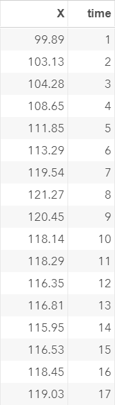
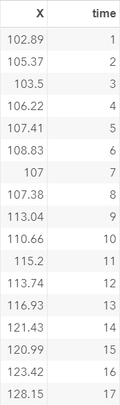
The EX2 data set contains a list of simulated values:
Let's again look at the time series profile using the ARIMA procedure.
proc arima data=ex2;
identify var=x;
run;
quit;
identify var=x;
run;
quit;
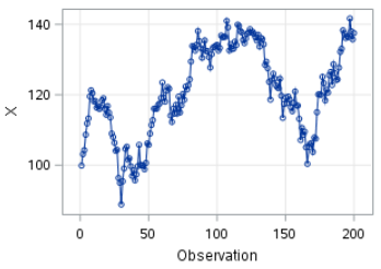
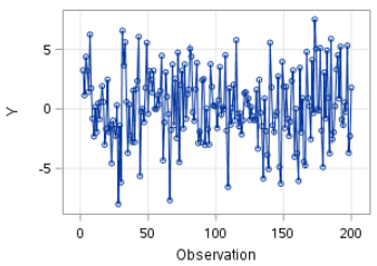
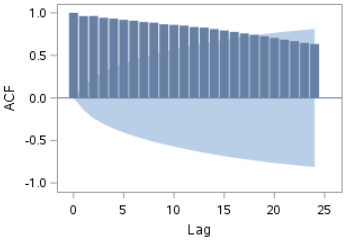
The time series plot clearly shows an upward and downward trend.
The mean of X does not stay constant over time:
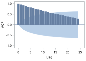
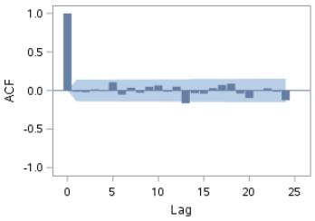
The ACF also shows a slow decline at longer lags:
One way to stationarize a time series is to do what we called differencing.
Differencing is subtraction of the variable X by its own lagged value.
Instead of modeling the movement of Xt, we will model the movement of Yt, where:
Yt = Xt - Xt-1
Let's look at an example.
data ex2a;
set ex2;
Y = dif(x);
run;
set ex2;
Y = dif(x);
run;
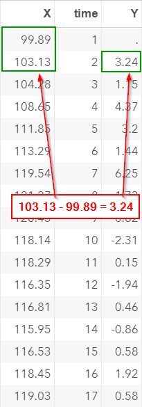
The DIF function in this example computes the difference between X and its own lagged value.
For example, X2 (i.e. X at time 2) is 103.13 and X1 is 99.89.
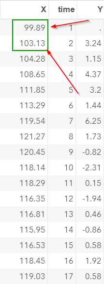
Y2 = X2 - X1 = 103.13 - 99.89 = 3.24
Differencing helps stabilize the mean of the time series.
Let's plot the time series, ACF and PACF on Y:
proc arima data=ex2a;
identify var=y;
run;
quit;
identify var=y;
run;
quit;
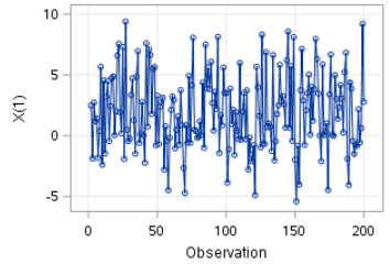
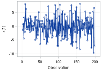
The time series plot for Y shows a constant mean.
It stays near 0 over time:
The ACF plot shows a sharp drop at lag 1.
The autocorrelation also seems to stay constant over time:
Nice! We have successfully transformed a non-stationary time series into a stationary time series.
Note: in this example, we have manually computed Y, which is the difference between X and its own lagged value.
This step is not necessary.
Differencing can be done in the ARIMA procedure.
Example
proc arima data=ex2;
identify var=x(1);
run;
quit;
identify var=x(1);
run;
quit;
We specified one in a bracket after the variable X (i.e. x(1)).
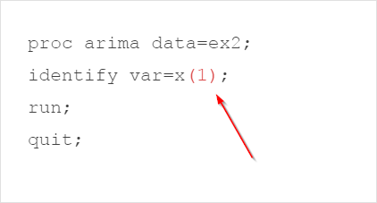
This tells SAS to perform one order of differencing.
The ARIMA procedure above will generate the exact same result as we had before (without manually computing Y).
(try it!)
Let's look at another example.
Copy and run the code from the yellow box below:
The EX3 data set again contains a list of simulated values for X:
We'll again run an ARIMA procedure on the EX3 data set:
proc arima data=ex3;
identify var=x;
run;
quit;
identify var=x;
run;
quit;
The time series plot shows a constant increase of X over time.
There is a clear upward trend that makes the series non-stationary.
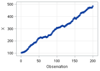
Again, we are going to stabilize the mean by one order of differencing.
proc arima data=ex3;
identify var=x(1);
run;
quit;
identify var=x(1);
run;
quit;
The series now shows a more stable mean:
Differencing does not always stationarize a series completely.
Let's look at the following example.
The EX4 data set also contains a list of simulated values.
proc arima data=ex4;
identify var=x;
run;
quit;
identify var=x;
run;
quit;
The movement of X is quite irregular.
It stays above 100 in the earlier part of the series before going below 100 in the later part of the plot.
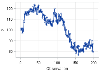
The ACF also shows a slow decline to zero.
This is another trait that shows the series is not stationary.
Now, let's perform our usual first order of differencing:
proc arima data=ex4;
identify var=x(1);
run;
quit;
identify var=x(1);
run;
quit;
The mean of the series is stabilized.
However, the ACF plot shows spikes at lags 1 and lag 2:
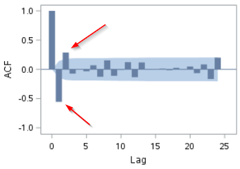
Overall, there is a huge improvement on stabilizing the mean of the series.
The spikes on the ACF plots will be modeled using additional parameters in the ARIMA model.
This will be discussed in the next few sections.
Exercise
If you haven't created the SALES3 data set, copy and run the code from the yellow box below:
If you haven't created the SALES3 data set, copy and run the code from the yellow box below:
Plot the ACF for the order type A (i.e. ORDERTYPEA variable).
Is the time series stationary?
Perform a one-order differencing if the series is not stationary. Do you see any improvement?
Need some help?
Fill out my online form.