Project 2 section 14

Search the site...

Sentry Page Protection

Time Series Modeling
[14-15]

The ESM procedure is another tool in SAS that allows you to perform quick forecasting using exponential smoothing.

If you haven't created the TS2 data set, copy and run the code from the yellow box below:

data ts2;
input time x;
datalines;
1 97.79
2 102.49
3 97.16
4 98.58
5 98.92
6 97.14
7 99.9
8 97.49
9 104.5
10 101.84
11 106.56
12 102.18
13 105.92
14 106.13
15 102.98
16 104.09
17 101.54
18 105.23
19 106.37
20 104.6
21 105.62
22 105.79
23 105.94
24 108.55
25 111.3
26 115.53
27 106.94
28 113.2
29 108.29
30 109.9
31 109.87
32 105
33 103.44
34 101.66
35 102.73
36 106.79
37 106
38 104.92
39 105.46
40 103.77
41 106.44
42 109.46
43 111.31
44 113.89
45 116.72
46 121.46
47 119.77
48 120.27
49 126.41
50 118.15
51 125.72
52 125.63
53 128.17
54 126.09
55 128.81
56 126.37
57 127.9
58 133.16
59 128.05
60 128.46
61 132.67
62 127.48
63 125.25
64 126.65
65 127.35
66 127.4
67 126.68
68 125.12
69 122.32
70 123.12
71 126.5
72 127.19
73 131.12
74 132.8
75 130.58
76 132.45
77 131.66
78 128.71
79 129.23
80 129.9
81 127.42
82 128.98
83 127.55
84 127.13
85 129.91
86 127.65
87 128.9
88 128.44
89 128.87
90 130.7
91 135.42
92 131.34
93 129.28
94 132.42
95 127.24
96 129.64
97 131.15
98 128.63
99 129.05
100 123.89
101 128.32
102 126.65
103 129.73
104 128.5
105 129.9
106 130.17
107 126.65
108 129.36
109 129.09
110 126.64
111 128.89
112 127.02
113 130.26
114 127.71
115 123.65
116 129.12
117 122.59
118 125.1
119 124.02
120 129.94
121 130.11
122 136.67
123 127.2
124 138.2
125 130.43
126 129.84
127 127.28
128 131.51
129 128.82
130 132.89
131 130.25
132 130.24
133 135.7
134 130.17
135 126.27
136 124.96
137 124.97
138 125.8
139 128.81
140 126.7
141 128.11
142 129.04
143 127.34
144 131.82
145 125.81
146 123.46
147 120.6
148 120.06
149 117.9
150 117.11
151 116.01
152 120.32
153 119.65
154 124.74
155 126.25
156 124.38
157 128.1
158 120.84
159 121.05
160 116.19
161 115.67
162 112.68
163 113.51
164 113.64
165 117.96
166 113.39
167 111.34
168 115.5
169 111.08
170 117
171 115.49
172 120.1
173 119.85
174 121.71
175 117.41
176 120.63
177 123.44
178 121.5
179 122.41
180 121.35
181 124.86
182 118.84
183 125.04
184 121.58
185 122.74
186 121.42
187 127.66
188 122.86
189 124.39
190 128.08
191 127.37
192 132.5
193 132.47
194 133.83
195 132.44
196 132.71
197 128
198 130.14
;
run;

Simple Exponential Smoothing

The Simple Exponential Smoothing (SES) model is equivalent to the ARIMA (0 1 1) model with no constant.

You can easily fit a SES model using the ESM procedure.

Example

proc esm data=ts2
back=14 lead=14
plot=(corr errors modelforecasts)
print=all;
forecast x / model=simple;
run;

The FORECAST statement in the ESM procedure tells SAS to perform forecasting.

The MODEL=SIMPLE simply specifies the model being the simple exponential smoothing.

The code above generates a number of tables and plots which includes:

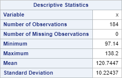
The Descriptive Statistics Table

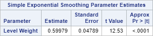
The Parameter Estimates Table

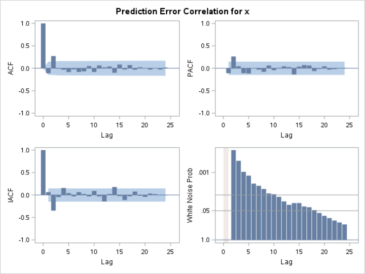
The Standard ACF and PACF Plots for Prediction Error

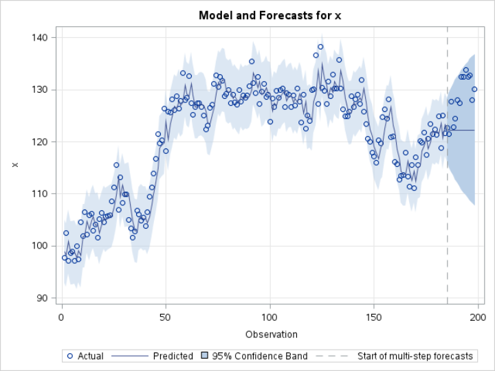
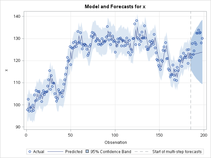
The Forecasting Plot for X

There are a number of additional models that can be fitted using the ESM procedure:

Simple Exponential Smoothing (model=simple)
Double Exponential Smoothing (model=double)
Linear (Holt) Exponential Smoothing (model=linear)
Damped Trend Exponential Smoothing (model=damptrend)
Additive Seasonal Exponential Smoothing (model=seasonal)
Multiplicative Seasonal Exponential Smoothing (model=addseasonal)
Winters Multiplicative Method (model=winters)
Winters Additive Method (model=addwinters)

Let's look at another example.

Linear (Holt) Exponential Smoothing

We are going to fit the Linear Exponential Smoothing model to the data.

proc esm data=ts2
back=14 lead=14
plot=(corr errors modelforecasts)
print=all;
forecast x / model=linear;
run;

Below is the forecasting plot from the Linear Exponential Smoothing model:

In the next (final) section, we will go back to the SALES data set from the very beginning, build an ARIMA model, and forecast the daily sales using 3-week forecasting periods.

Exercise

Perform damped trend exponential smoothing on the TS2 data set.

Need some help?

Fill out my online form.