Sentry Page Protection
Time Series Modeling
[15-15]
[15-15]
In this section, we will go back to the SALES data set we worked on in the beginning.
We will build an ARIMA model to forecast the total sales based on the sales record over the 60-day period.
If you haven't created the SALES3 data set, copy and run the code from the yellow box below:
We will first use the ARIMA procedure to check whether there is autocorrelation in the time series.
proc arima data=sales3;
identify var=totalsales;
run;
quit;
identify var=totalsales;
run;
quit;
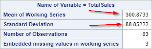
From the descriptive statistics, we see that there are 63 observations in the SALES3 data set with three missing values.
The average daily sales is around $300 with a standard deviation of 88.85.
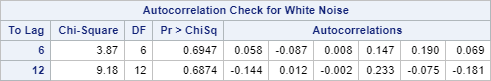
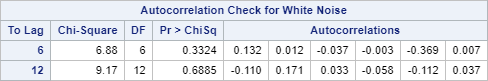
The p-values from the Ljung-box test are above 0.05 at lag 6 and 12.
This concludes that the series is purely white noise:
Since the time series does not show any systematic pattern, we could simply assume the daily sales resolves around $300 with a standard deviation of $88.85.
The future daily sales are predicted to be $300 for the foreseeable future.
This is the same as fitting an ARIMA (0 0 0) model to the data with no differencing, AR or MA term.
We will now add an ESTIMATE statement to the ARIMA procedure and look at the results:
proc arima data=sales3;
identify var=totalsales noprint;
estimate;
run;
quit;
identify var=totalsales noprint;
estimate;
run;
quit;
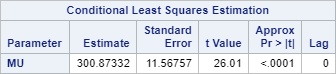
The parameter estimate for µ (mean) is $300.83.
This is the mean of the entire time series:
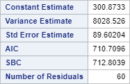
The AIC and SBC are 710.7096 and 712.8039, respectively.
Now, let's perform the forecasting and compute the RMSE:
proc arima data=sales3;
identify var=totalsales noprint;
estimate noprint;
forecast back=15 lead=15 out=out_pred1;
run;
quit;
data test;
set out_pred1;
if _n_ >=49;
run;
proc sql;
select mean(abs(totalsales-forecast)) format 20.10 as mae,
sqrt(mean((totalsales-forecast)**2)) format 20.10 as rmse from test;
quit;
identify var=totalsales noprint;
estimate noprint;
forecast back=15 lead=15 out=out_pred1;
run;
quit;
data test;
set out_pred1;
if _n_ >=49;
run;
proc sql;
select mean(abs(totalsales-forecast)) format 20.10 as mae,
sqrt(mean((totalsales-forecast)**2)) format 20.10 as rmse from test;
quit;
Scroll down to the bottom of the output.
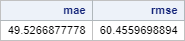
The MAE and RMSE are 49.53 and 60.46, respectively.
The MAE and RMSE are 49.53 and 60.46, respectively.
Are we done? Can we get a better model?
Let's look at the residual, which is the difference between the actual value and the predicted value.
proc sql;
select totalsales, forecast, residual
from test;
quit;
select totalsales, forecast, residual
from test;
quit;
You can see that some residuals are fairly large.
Some of the sales predictions are off by more than $100.
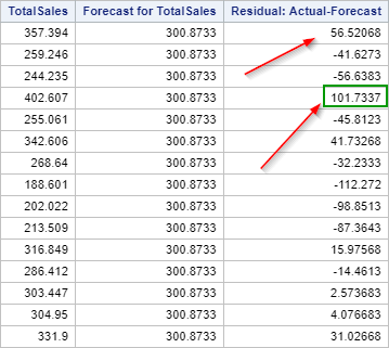
Maybe there is a model that does a better job in the sales forecast.
In section 2, we have learned that Monday's sales are substantially higher than the rest of the week.
We can model this seasonal spike by having a seasonal differencing of 5 days.
proc arima data=sales3;
identify var=totalsales(5);
estimate;
forecast back=15 lead=15 out=out_pred2;
run;
quit;
identify var=totalsales(5);
estimate;
forecast back=15 lead=15 out=out_pred2;
run;
quit;
Adding a seasonal differencing of 5 days to the model will change the outlook of the ACF and PACF plots.
Let's look at the tables generated.
The p-values from the Ljung-box test are still at an insignificant level:
This is good.
Let's look at the ACF and PACF plots:
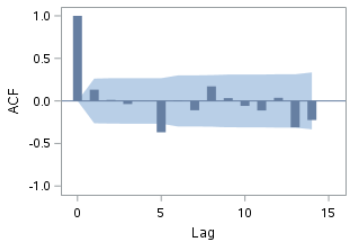
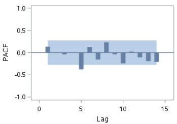
Both plots show a spike at lag 5. However, based on the Ljung-box test, we cannot reject the null hypothesis that the residuals are white noise.
The residual plots look worse. However, let's look at the AIC and SBC:
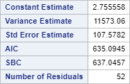
The AIC and SBC are 635.0945 and 634.0457, respectively.
These are much lower (better) than the earlier model where AIC=710.7096 and SBC=712.8039.
Now, let's look at the residuals as well as the RMSE:
proc arima data=sales3;
identify var=totalsales(5) noprint;
estimate noprint;
forecast back=15 lead=15 out=out_pred2;
run;
quit;
data test;
set out_pred2;
if _n_ >=49;
run;
proc sql;
select mean(abs(totalsales-forecast)) format 20.10 as mae,
sqrt(mean((totalsales-forecast)**2)) format 20.10 as rmse from test;
quit;
identify var=totalsales(5) noprint;
estimate noprint;
forecast back=15 lead=15 out=out_pred2;
run;
quit;
data test;
set out_pred2;
if _n_ >=49;
run;
proc sql;
select mean(abs(totalsales-forecast)) format 20.10 as mae,
sqrt(mean((totalsales-forecast)**2)) format 20.10 as rmse from test;
quit;
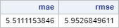
Again, scroll to the very bottom.
The MAE and RMSE are much lower!
They are now at 5.51 and 5.95 as opposed to 49.53 and 60.46 from the earlier model.
The residuals also look great!
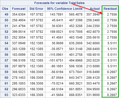
The residuals are mostly under 10. The sales forecast is off by less than 10 at each of the time points.
Note: the residuals look too clean to be real. We suspect the sales data set might have been systematically generated, as opposed to being obtained as an actual sales record of a business.
Done! The ARIMA model we have identified is the Seasonal ARIMA (0 0 0) (0 1 0)5.