Sentry Page Protection
Time Series Modeling
[7-15]
[7-15]
Introduction to ARIMA Modeling
Now that we have learned how to plot and interpret the ACF and PACF of a time series, let's look at an overview of how to build an ARIMA model.
ARIMA stands for Autoregressive Integrated Moving Average. It consists of three components:
- AR Term
- Differencing Order
- MA Term
We will learn more about each component shortly.
The first step to building an ARIMA model is to examine whether the series is stationary.
Stationarity
A time series is said to be stationary if it has a constant expected value (i.e. mean), variance and autocorrelation.
The statistical properties of the time series do not change over time.
Let's look at an example of a stationary time series:
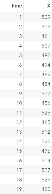
The EX1 data set contains a list of simulated values for X over a period of 200 days.
Now, we are going to look at the profile of the time series using the ARIMA procedure.
Example
proc arima data=ex1;
identify var=x;
run;
quit;
identify var=x;
run;
quit;
The ARIMA procedure is a more versatile tool than the TIMESERIES procedure.
The IDENTIFY statement in Proc ARIMA is used during the initial exploration stage.
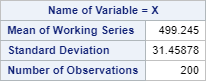
In our example, it computes the descriptive statistics of X:
The descriptive statistics below is the white noise test result, which we will discuss shortly:

It also shows the time series for the ACF, PACF and IACF plots:
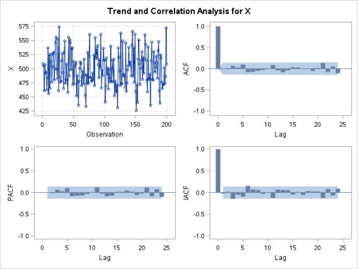
These plots and tables often contain enough information for you to decide whether the time series is stationary or not.
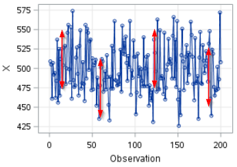
Let's look at the time series plot.
The time series plot shows that the mean of X stays close to 500 over the entire period.
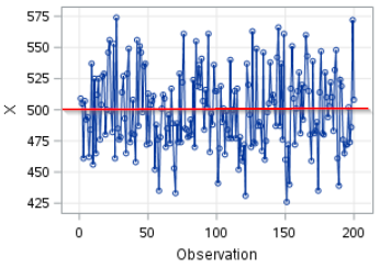
The variance stays constant over time:
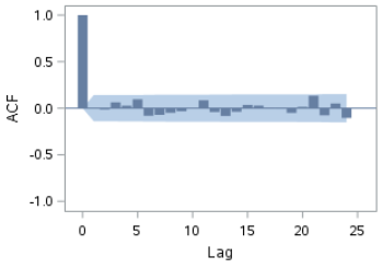
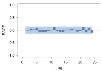
The autocorrelations are weak in both the ACF and PACF plots:
The ARIMA procedure also performs the Ljung-box test, which is a hypothesis testing of whether the series is simply white noise.
It tests whether the autocorrelation is significantly different from zero.
The Ljung-box test results are displayed as the Autocorrelation Check for White Noise table:
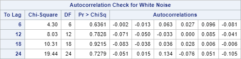
In the table, the p-values are above 0.05 at lags 6, 12, 18 and 24.
We failed to reject the hypothesis that the data is just white noise.
All of these are the properties of a stationary time series.
Why stationary?
In general, we want the time series to be stationary.
It is easier to forecast the future when the expected results don't change much over time.
For example, let's assume the average daily sales over the last 60 days is roughly $500, and it usually ranges between $400 to $600.
When doing the sales forecast, you would likely expect the future sales to be, on average, $500 and within the range of $400 to $600 as well.
Unfortunately, in practice, time series are rarely stationary.
Its expected value usually moves up and down with different degrees of fluctuation during different periods.
The general approach to time series modeling is to transform the non-stationary time series into an approximate stationary time series.
We then fit a model to the transformed time series, and perform the forecasting on the stationary series.
Let's look at some examples of the non-stationary time series.
Example 1: Non-constant mean
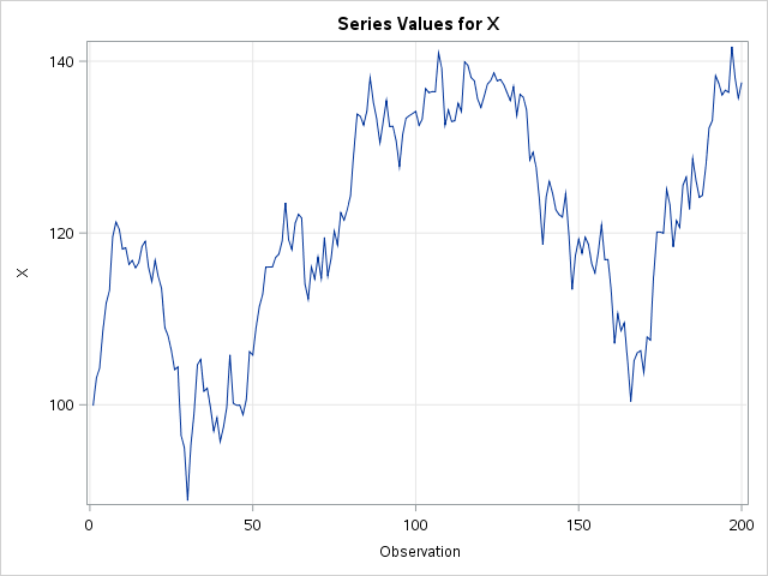
This time series is not stationary.
The mean of X goes up and down, and it does not stay constant.
This is a trait of a non-stationary time series.
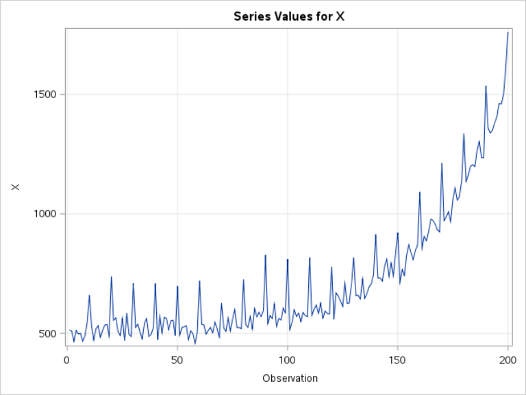
Example 2: Non-constant mean
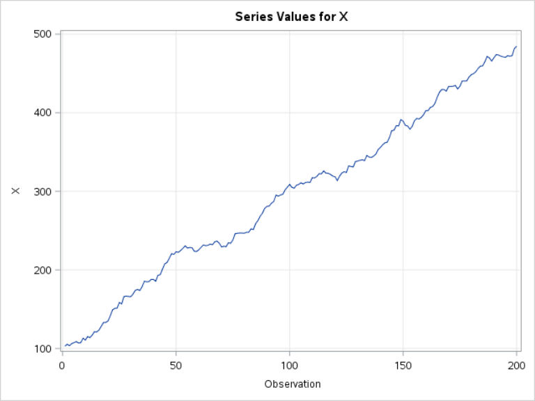
A time series with any upward or downward trend is, by definition, not stationary.
Its mean again does not stay constant over time.
Example 3: Non-constant mean
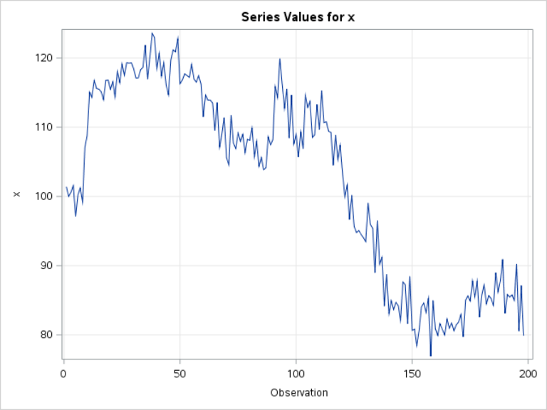
This time series, again, does not have a constant mean. It is not a stationary series.
Example 4: Increasing variance
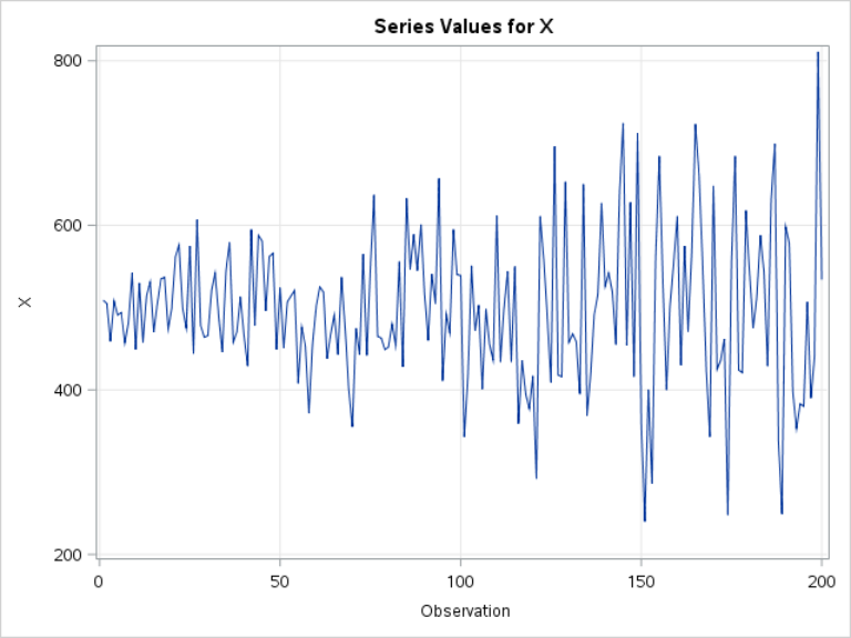
This time series plot shows increasing variance. This is also a trait of non-stationary time series.
Example 5: Seasonal Cycle
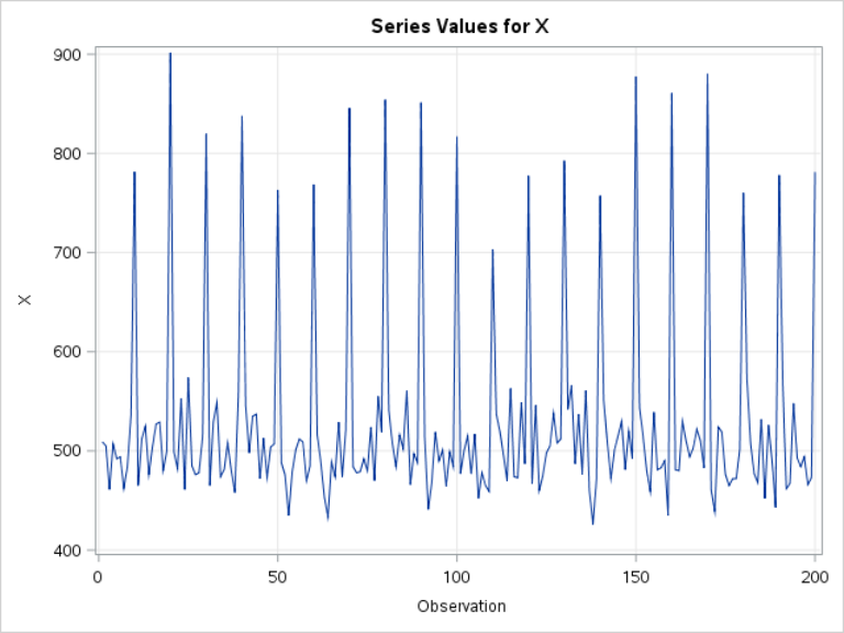
There are seasonal spikes every 10 days.
The mean at these spikes is much higher than other days.
This is, by definition, not a stationary time series.
A time series with a non-constant mean can often be stationarized by differencing.
Unequal variance can sometimes be stabilized by transformation.
Seasonal time series can often be transformed into a stationary series by seasonal differencing.
We will be looking at some examples in the next section.
Exercise
Take a look at the time series plot below.
Take a look at the time series plot below.
Is this a stationary time series? Why or why not?
Need some help?
Fill out my online form.