Sentry Page Protection
Time Series Modeling
[11-15]
[11-15]
Differencing or transformation do not always remove all of the autocorrelation from the time series.
Let's look at an example.
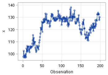
The TS2 data set is another non-stationary time series.
Let's plot the X column on a time series plot:
proc arima data=ts2;
identify var=x;
run;
quit;
identify var=x;
run;
quit;
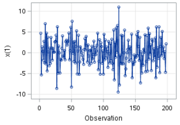
Let's look at the results with one order of differencing.
proc arima data=ts2;
identify var=x(1);
run;
quit;
identify var=x(1);
run;
quit;
The time series plot looks good. The random movement has been removed:
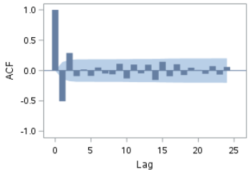
However, the ACF (after differencing) shows spikes at lags 1 and 2:
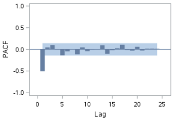
The PACF also shows a spike at lag 1:
Let's look at the Ljung-box test result.
The p-values at all four lags are less than 0.0001. We reject the null hypothesis that the residuals are white noise.
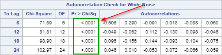
There is remaining autocorrelation left in the residual that is not explained by our model.
Now, what are we going to do next?
The PACF plot of the residual shows a spike at lag 1.
This indicates that the residual at time t is highly correlated with itself at time (t-1).
We can try adding an AR term to the model and see if it improves the residual.
Brief Introduction to the AR Model
The AR (Autoregressive) model models the time series (X) based on the previous value of X (i.e. Xt-1).
With just one AR term, it has the following forecasting equation:
Xt = µ + ϕ1Xt-1 + Wt
With two AR terms, it has an additional term in the equation:
Xt = µ + ϕ1Xt-1 + ϕ2Xt-2 + Wt
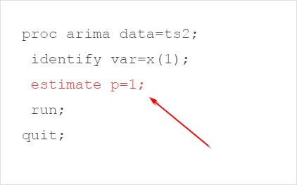
Let's add an AR term to the model and see if it improves the autocorrelation in the residuals.
proc arima data=ts2;
identify var=x(1);
estimate p=1;
run;
quit;
identify var=x(1);
estimate p=1;
run;
quit;
We have added an ESTIMATE statement with the p=(1) option.
This specifies the number of AR terms (p).
There are many results generated.
Let's look at each of them individually.
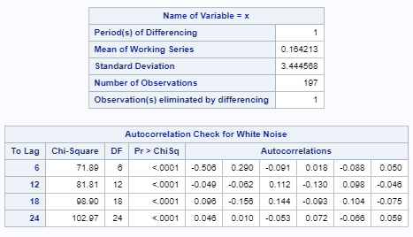
The first set of tables are the Ljung-box test results before adding the AR term.
We have seen these results earlier:
There are a number of tables that have important statistics.
Let's look at the Conditional Least Squares Estimation table:
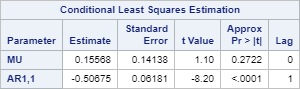
It shows the estimates for the µ and ϕ1 from the forecasting equation:
Xt = µ + ϕ1Xt-1 + Wt
The p-value for (AR1, 1) is less than 0.0001. This indicates the parameter estimate is significantly different from zero.
The next table shows the AIC and SBC for the model.
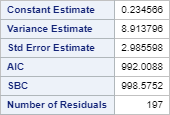
AIC and SBC are used for model comparison purposes.
The lower the AIC and/or SBC, the better.
We will look at some examples shortly.
The below shows the Autocorrelation Check of Residuals:
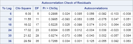
These are the Ljung-box test results after adding the AR term.
The p-values at each lag are above 0.05.
We're done! We conclude that the residuals after adding the AR term are now just white noise.
The model we have identified is ARIMA (1 1 0).
It has one AR term with one order of differencing.
Now, how do we know the ARIMA (1 1 0) model is better than the ARIMA (0 1 0) model that we had earlier?
There are a number of ways to perform a model comparison.
One common way to select a model is to compare the AIC and SBC values.
The model with the lower AIC and SBC are usually the better model.
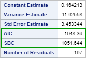
Let's look at the AIC and SBC from the ARIMA (0 1 0) model:
proc arima data=ts2 plots=none;
identify var=x(1) noprint;
estimate;
run;
quit;
identify var=x(1) noprint;
estimate;
run;
quit;
The AIC and SBC for ARIMA (0 1 0) is 1048.36 and 1051.644, respectively.
Now, let's look at the AIC and SBC for the ARIMA (1 1 0) model:
proc arima data=ts2 plots=none;
identify var=x(1) noprint;
estimate p=1;
run;
quit;
identify var=x(1) noprint;
estimate p=1;
run;
quit;
The AIC and SBC are 992.0088 and 998.5752, respectively.
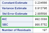
Based on the AIC and SBC, the ARIMA (1 1 0) is the better model among of two.
Another issue with the ARIMA (0 1 0) model, as we have mentioned before, is that its residual shows remaining autocorrelation that is not explained by the model.
This indicates that there is a systematic pattern that could be explained by additional AR / MA terms.
In the next section, we will look at an example where adding an MA term could improve the model from the stationarized time series.
Exercise
Copy and run the ORDER data set from the yellow box below:
Copy and run the ORDER data set from the yellow box below:
The ORDER data set contains the number of orders for a period of 100 days.
Perform the necessary steps to identify one ARIMA model where the residuals are purely white noise.
Need some help?
Fill out my online form.