Sentry Page Protection
Time Series Modeling
[12-15]
[12-15]
In this section, we are going to look at an example of how an MA term can correct the autocorrelation in the residuals.
Copy and run the code from the yellow box below:
We are going to run the Proc ARIMA to display all of the plots and Ljung-box test for the time series:
proc arima data=ts3 ;
identify var=x;
run;
quit;
identify var=x;
run;
quit;
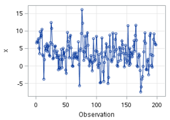
The time series plot shows the mean is fairly stable.
Differencing might not be needed.
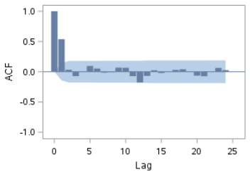
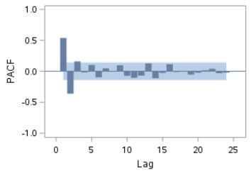
The ACF and PACF show spikes at various lags:
Also, the p-values from the Ljung-box test are significant at each of the four lags.
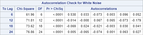
This indicates the data is autocorrelated. An AR or MA term can be used to model the autocorrelation.
Let's try adding an AR term:
proc arima data=ts3 ;
identify var=x;
estimate p=1;
run;
quit;
identify var=x;
estimate p=1;
run;
quit;
The parameter estimate is significant at lag 1:
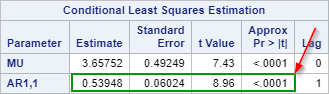
However, the Ljung-box test (i.e. white noise test) still shows significant results at each lag values:
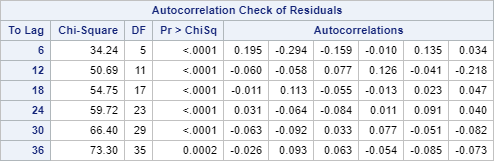
There is unexplained correlation in the residuals even after adding one AR term to the model.
Now, let's try adding two AR terms.
proc arima data=ts3 ;
identify var=x;
estimate p=2;
run;
quit;
identify var=x;
estimate p=2;
run;
quit;
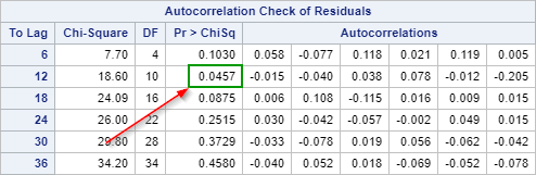
There is an improvement on the Ljung-box test. However, there is still a significant p-value at lag 12:
In general, the lag where ACF plot drops off indicates the number of MA terms for the model.
In this example, the ACF plot drops off after lag 1:
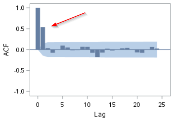
This indicates the autocorrelation could possibly be explained by an MA term.
Brief Introduction to an MA Model
The MA (Moving Average) model models the time series (X) based on the previous error of X (i.e. Wt-1).
With just one MA term, it has the following forecasting equation:
Xt = µ + Wt + ϕ1Wt-1
With two MA terms, it has an additional term in the equation:
Xt = µ + Wt + ϕ1Wt-1 + ϕ2Wt-2
Let's add an MA term to the model to see if it explains the autocorrelation in the residuals.
proc arima data=ts3 ;
identify var=x;
estimate q=1;
run;
quit;
identify var=x;
estimate q=1;
run;
quit;
There is a huge improvement on the Ljung-box test.
The p-values are insignificant at each lag level:
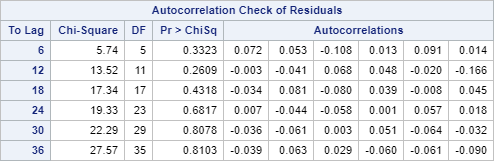
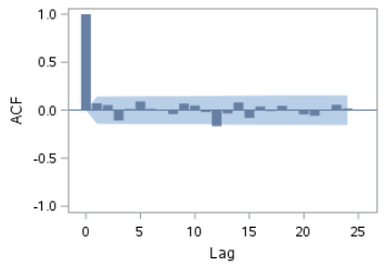
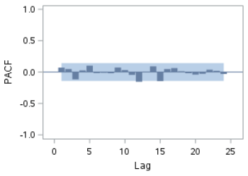
The ACF and PACF plots show a small spike at lag 12.
However, since the Ljung-box test fails to reject the hypothesis that the time series is white noise, we can conclude that the autocorrelation in the residuals is insignificant.
Done! We have identified the model for the data to be ARIMA (0 0 1) (i.e.an MA(1) model).
In the following sections, we will learn how to do forecasting with the models we have built so far.
Note: identifying the right number of AR and/or MA terms is a complex and intuitive process.
For an in-depth tutorial on this topic, please visit this site.
Exercise
Copy and run the EXER data set from the yellow box below:
Copy and run the EXER data set from the yellow box below:
Perform the necessary steps to identify one ARIMA model where the residuals are purely white noise.
Need some help?
Fill out my online form.